Sección 13 Ejemplos de inferencia bayesiana en Stan I
En esta parte veremos cómo correr y diagnosticar en Stan varios ejemplos vistos en clase. Para instalar cmdstanr y Stan, puedes ver aquí. En python puedes usar pystan, por ejemplo.
# install.packages("cmdstanr", repos = c("https://mc-stan.org/r-packages/", getOption("repos")))
library(cmdstanr)
library(posterior)
library(tidyverse)
library(bayesplot)
Hay dos pasos escenciales para hacer análisis con Stan: 1) Definir la estructura del modelo usando notacion de stan (recomendado hacerlo en un archivo de texto independiente) y 2) simular de la posterior.
Al definir la estructura debemos especificar 3 aspectos:
Los datos (
data): son las observaciones, a diferencia de R, stan es un lenguaje ti hay cotas y la dimensión de los vectores o matrices.ros o reales, también establecemos si hay cotas y la dimensión de los vectores, matrices o valores.Los parámetrros (
parameters) de los que depende el modelo, nuevamente especificando dimensión, si es acotado y el tipo de dato. parameters.El modelo (
model), especificamos la verosimilitud y las inciales.
Veamos el ejemplo beta biomial para la estimación de una proporción
Estimación de una proporción
Escribimos el código para el modelo en un archivo modelo-1.stan, y compilamos:
archivo_stan <- file.path("stan/modelo-1.stan")
# compilar
mod <- cmdstan_model(archivo_stan)mod## // Ejemplo de estimación de una proporcion
## data {
## int n; // número de pruebas
## int y; //numero de éxitos y fracasos
## }
##
## parameters {
## real<lower=0,upper=1> theta;
## }
##
## model {
## // inicial
## theta ~ beta(3, 3);
## y ~ binomial(n, theta);
## }Pasamos datos y muestreamos
datos_lista <- list(n = 30, y = 19)
ajuste <- mod$sample(
  data = datos_lista,
  seed = 1234,
  chains = 4,
  parallel_chains = 4,
  refresh = 300)
## Running MCMC with 4 parallel chains...
##
## Chain 1 Iteration: 1 / 2000 [ 0%] (Warmup)
## Chain 1 Iteration: 300 / 2000 [ 15%] (Warmup)
## Chain 1 Iteration: 600 / 2000 [ 30%] (Warmup)
## Chain 1 Iteration: 900 / 2000 [ 45%] (Warmup)
## Chain 1 Iteration: 1001 / 2000 [ 50%] (Sampling)
## Chain 1 Iteration: 1300 / 2000 [ 65%] (Sampling)
## Chain 1 Iteration: 1600 / 2000 [ 80%] (Sampling)
## Chain 1 Iteration: 1900 / 2000 [ 95%] (Sampling)
## Chain 1 Iteration: 2000 / 2000 [100%] (Sampling)
## Chain 2 Iteration: 1 / 2000 [ 0%] (Warmup)
## Chain 2 Iteration: 300 / 2000 [ 15%] (Warmup)
## Chain 2 Iteration: 600 / 2000 [ 30%] (Warmup)
## Chain 2 Iteration: 900 / 2000 [ 45%] (Warmup)
## Chain 2 Iteration: 1001 / 2000 [ 50%] (Sampling)
## Chain 2 Iteration: 1300 / 2000 [ 65%] (Sampling)
## Chain 2 Iteration: 1600 / 2000 [ 80%] (Sampling)
## Chain 2 Iteration: 1900 / 2000 [ 95%] (Sampling)
## Chain 2 Iteration: 2000 / 2000 [100%] (Sampling)
## Chain 3 Iteration: 1 / 2000 [ 0%] (Warmup)
## Chain 3 Iteration: 300 / 2000 [ 15%] (Warmup)
## Chain 3 Iteration: 600 / 2000 [ 30%] (Warmup)
## Chain 3 Iteration: 900 / 2000 [ 45%] (Warmup)
## Chain 3 Iteration: 1001 / 2000 [ 50%] (Sampling)
## Chain 3 Iteration: 1300 / 2000 [ 65%] (Sampling)
## Chain 3 Iteration: 1600 / 2000 [ 80%] (Sampling)
## Chain 3 Iteration: 1900 / 2000 [ 95%] (Sampling)
## Chain 3 Iteration: 2000 / 2000 [100%] (Sampling)
## Chain 4 Iteration: 1 / 2000 [ 0%] (Warmup)
## Chain 4 Iteration: 300 / 2000 [ 15%] (Warmup)
## Chain 4 Iteration: 600 / 2000 [ 30%] (Warmup)
## Chain 4 Iteration: 900 / 2000 [ 45%] (Warmup)
## Chain 4 Iteration: 1001 / 2000 [ 50%] (Sampling)
## Chain 4 Iteration: 1300 / 2000 [ 65%] (Sampling)
## Chain 4 Iteration: 1600 / 2000 [ 80%] (Sampling)
## Chain 4 Iteration: 1900 / 2000 [ 95%] (Sampling)
## Chain 4 Iteration: 2000 / 2000 [100%] (Sampling)
## Chain 1 finished in 0.0 seconds.
## Chain 2 finished in 0.0 seconds.
## Chain 3 finished in 0.0 seconds.
## Chain 4 finished in 0.0 seconds.
##
## All 4 chains finished successfully.
## Mean chain execution time: 0.0 seconds.
## Total execution time: 0.3 seconds.Checamos diagnósticos:
ajuste$cmdstan_diagnose()## Checking sampler transitions treedepth.
## Treedepth satisfactory for all transitions.
##
## Checking sampler transitions for divergences.
## No divergent transitions found.
##
## Checking E-BFMI - sampler transitions HMC potential energy.
## E-BFMI satisfactory.
##
## Rank-normalized split effective sample size satisfactory for all parameters.
##
## Rank-normalized split R-hat values satisfactory for all parameters.
##
## Processing complete, no problems detected.Si no hay problemas, podemos ver el resumen:
ajuste$summary()## # A tibble: 2 × 10
## variable mean median sd mad q5 q95 rhat ess_bulk ess_tail
## <chr> <dbl> <dbl> <dbl> <dbl> <dbl> <dbl> <dbl> <dbl> <dbl>
## 1 lp__ -24.6 -24.3 0.729 0.324 -26.1 -24.1 1.00 2071. 2263.
## 2 theta 0.614 0.617 0.0809 0.0817 0.475 0.741 1.00 1574. 1995.Donde verificamos que el tamaño de muestra efectivo (ess) y el diagnóstico de \(\hat{R}\) son apropiados.
Adicional a los bloques de data, parameters y model hay opciones que nos dan
más funcionalidad, por ejemplo generated quantities. Este bloque se puede utlizar
para simular de una distribución dada (como abajo), de la predictiva posterior o
para transformar la salida. Corre después de cada iteración.
Usémoslo para simular de la incial.
archivo_stan <- file.path("stan/modelo-1b.stan")
# compilar
mod <- cmdstan_model(archivo_stan)mod## // Ejemplo de estimación de una proporcion
## data {
## int n; // número de pruebas
## int y; //numero de éxitos y fracasos
## }
##
## parameters {
## real<lower=0,upper=1> theta;
## }
##
## model {
## // inicial
## theta ~ beta(3, 3);
## y ~ binomial(n, theta);
## }
##
## generated quantities {
## real theta_inicial;
## theta_inicial = beta_rng(3, 3);
## }Podemos ver las cadenas de la siguiente forma:
ajuste <- mod$sample(
  data = datos_lista,
  seed = 1234,
  chains = 4,
  parallel_chains = 4,
  refresh = 500)
## Running MCMC with 4 parallel chains...
##
## Chain 1 Iteration: 1 / 2000 [ 0%] (Warmup)
## Chain 1 Iteration: 500 / 2000 [ 25%] (Warmup)
## Chain 1 Iteration: 1000 / 2000 [ 50%] (Warmup)
## Chain 1 Iteration: 1001 / 2000 [ 50%] (Sampling)
## Chain 1 Iteration: 1500 / 2000 [ 75%] (Sampling)
## Chain 1 Iteration: 2000 / 2000 [100%] (Sampling)
## Chain 2 Iteration: 1 / 2000 [ 0%] (Warmup)
## Chain 2 Iteration: 500 / 2000 [ 25%] (Warmup)
## Chain 2 Iteration: 1000 / 2000 [ 50%] (Warmup)
## Chain 2 Iteration: 1001 / 2000 [ 50%] (Sampling)
## Chain 2 Iteration: 1500 / 2000 [ 75%] (Sampling)
## Chain 2 Iteration: 2000 / 2000 [100%] (Sampling)
## Chain 3 Iteration: 1 / 2000 [ 0%] (Warmup)
## Chain 3 Iteration: 500 / 2000 [ 25%] (Warmup)
## Chain 3 Iteration: 1000 / 2000 [ 50%] (Warmup)
## Chain 3 Iteration: 1001 / 2000 [ 50%] (Sampling)
## Chain 3 Iteration: 1500 / 2000 [ 75%] (Sampling)
## Chain 3 Iteration: 2000 / 2000 [100%] (Sampling)
## Chain 4 Iteration: 1 / 2000 [ 0%] (Warmup)
## Chain 4 Iteration: 500 / 2000 [ 25%] (Warmup)
## Chain 4 Iteration: 1000 / 2000 [ 50%] (Warmup)
## Chain 4 Iteration: 1001 / 2000 [ 50%] (Sampling)
## Chain 4 Iteration: 1500 / 2000 [ 75%] (Sampling)
## Chain 4 Iteration: 2000 / 2000 [100%] (Sampling)
## Chain 1 finished in 0.0 seconds.
## Chain 2 finished in 0.0 seconds.
## Chain 3 finished in 0.0 seconds.
## Chain 4 finished in 0.0 seconds.
##
## All 4 chains finished successfully.
## Mean chain execution time: 0.0 seconds.
## Total execution time: 0.2 seconds.theta_tbl <- ajuste$draws(c("theta", "theta_inicial")) |> as_draws_df()
# Podemos graficar manual
ggplot(theta_tbl, aes(x = .iteration, y = theta)) +
geom_line() +
facet_wrap(~.chain, ncol = 1)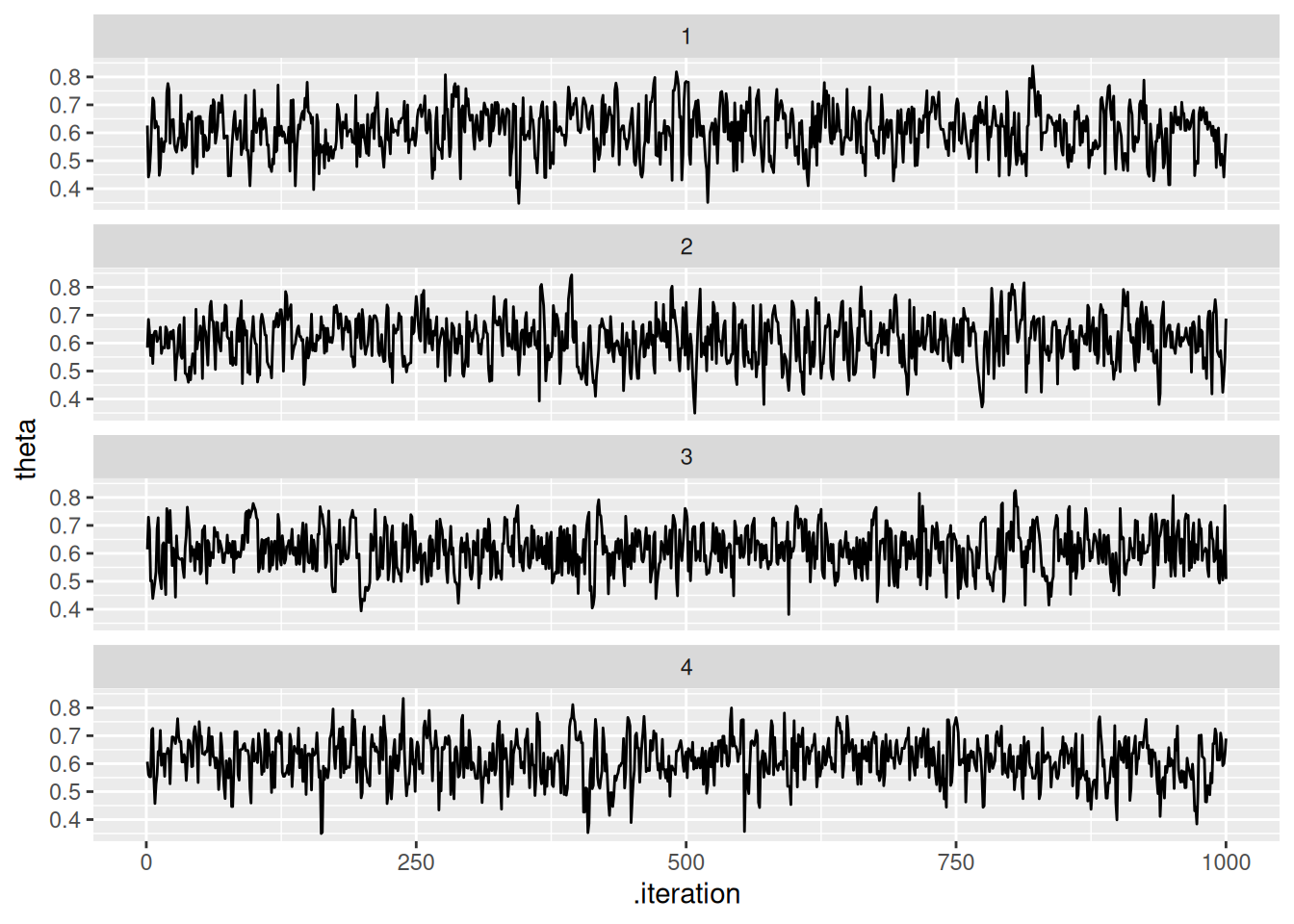
# O podemos usar las funciones del paquete bayesplot
mcmc_trace(ajuste$draws(c("theta")))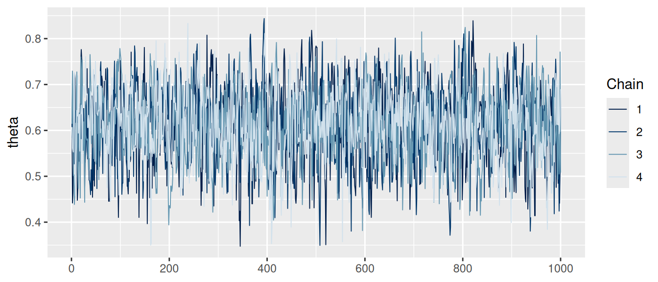
Y replicamos la gráfica de las notas haciendo:
sims_tbl <- theta_tbl |> pivot_longer(theta:theta_inicial, names_to = "dist", values_to = "theta")## Warning: Dropping 'draws_df' class as required metadata was removed.ggplot(sims_tbl, aes(x = theta, fill = dist)) +
geom_histogram(aes(x = theta), bins = 30, alpha = 0.5, position = "identity")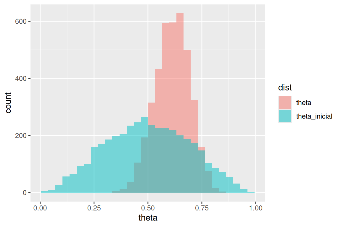
Nota, hay muchas funciones útiles en bayesplot.
# Histogramas y densidades
mcmc_hist(ajuste$draws(c("theta", "theta_inicial"))) +
  yaxis_text(TRUE) +
  ylab("count")
## `stat_bin()` using `bins = 30`. Pick better value `binwidth`.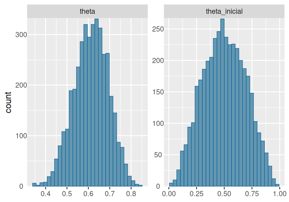
mcmc_dens(ajuste$draws(), pars = c("theta", "theta_inicial")) +
  yaxis_text(TRUE) +
  ylab("density")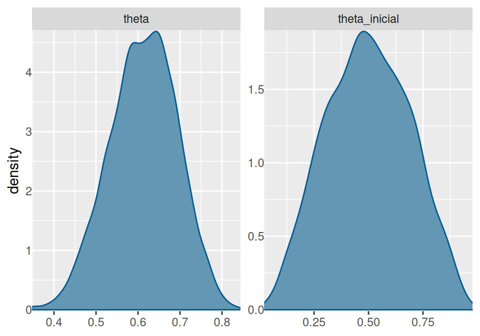
# Densidades por cadena
mcmc_dens_overlay(ajuste$draws(c("theta", "theta_inicial"))) +
  ylab("count")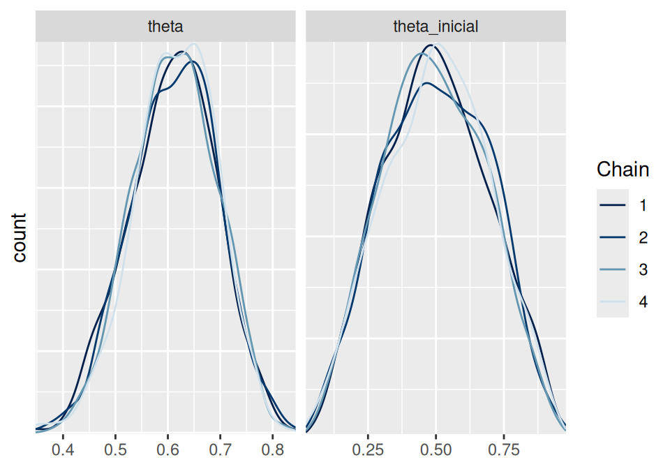
# ACF
mcmc_acf(ajuste$draws(c("theta", "theta_inicial"))) 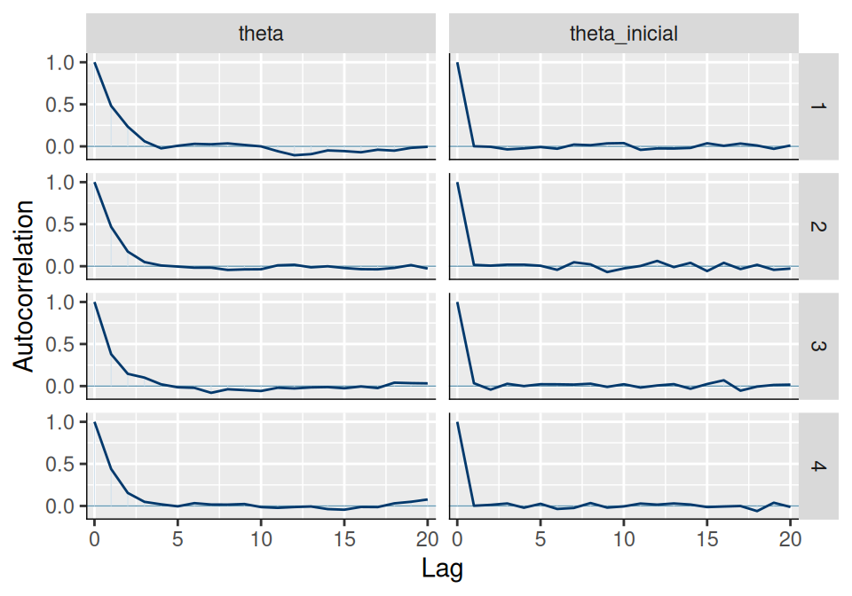
Estimación del máximo de una uniforme
Tomamos el ejemplo de los boletos de lotería,
loteria_tbl <- read_csv("data/nums_loteria_avion.csv", col_names = c("id", "numero")) |>
  mutate(numero = as.integer(numero))
## Rows: 99 Columns: 2
## ── Column specification ────────────────────────────────────────────────────────
## Delimiter: ","
## chr (1): numero
## dbl (1): id
##
## ℹ Use `spec()` to retrieve the full column specification for this data.
## ℹ Specify the column types or set `show_col_types = FALSE` to quiet this message.set.seed(334)
muestra_loteria <- sample_n(loteria_tbl, 25) |>
mutate(numero = numero/1000)mod## // Ejemplo de estimación del máximo de uniforme
## data {
## int n; // número de observaciones
## array[n] real y; //datos observados
## }
##
## transformed data{
## real y_max;
## y_max = max(y);
## }
##
## parameters {
## real<lower=y_max> theta;
## }
##
## model {
## // inicial
## theta ~ pareto(300, 1.1);
## y ~ uniform(0, theta);
## }Pasamos datos y muestreamos:
datos_lista <- list(n = nrow(muestra_loteria), y = muestra_loteria$numero)
ajuste <- mod$sample(
  data = datos_lista,
  seed = 1234,
  chains = 4,
  iter_warmup = 5000,
  iter_sampling = 20000,
  parallel_chains = 4,
  refresh = 5000)
## Running MCMC with 4 parallel chains...
##
## Chain 1 Iteration: 1 / 25000 [ 0%] (Warmup)
## Chain 1 Iteration: 5000 / 25000 [ 20%] (Warmup)
## Chain 1 Iteration: 5001 / 25000 [ 20%] (Sampling)
## Chain 1 Iteration: 10000 / 25000 [ 40%] (Sampling)
## Chain 1 Iteration: 15000 / 25000 [ 60%] (Sampling)
## Chain 2 Iteration: 1 / 25000 [ 0%] (Warmup)
## Chain 2 Iteration: 5000 / 25000 [ 20%] (Warmup)
## Chain 2 Iteration: 5001 / 25000 [ 20%] (Sampling)
## Chain 2 Iteration: 10000 / 25000 [ 40%] (Sampling)
## Chain 2 Iteration: 15000 / 25000 [ 60%] (Sampling)
## Chain 3 Iteration: 1 / 25000 [ 0%] (Warmup)
## Chain 3 Iteration: 5000 / 25000 [ 20%] (Warmup)
## Chain 3 Iteration: 5001 / 25000 [ 20%] (Sampling)
## Chain 3 Iteration: 10000 / 25000 [ 40%] (Sampling)
## Chain 3 Iteration: 15000 / 25000 [ 60%] (Sampling)## Chain 3 Informational Message: The current Metropolis proposal is about to be rejected because of the following issue:## Chain 3 Exception: uniform_lpdf: Upper bound parameter is inf, but must be finite! (in '/tmp/RtmpBTfO0T/model-4dbc4bf964c9.stan', line 19, column 2 to column 24)## Chain 3 If this warning occurs sporadically, such as for highly constrained variable types like covariance matrices, then the sampler is fine,## Chain 3 but if this warning occurs often then your model may be either severely ill-conditioned or misspecified.## Chain 3## Chain 4 Iteration: 1 / 25000 [ 0%] (Warmup)
## Chain 4 Iteration: 5000 / 25000 [ 20%] (Warmup)
## Chain 4 Iteration: 5001 / 25000 [ 20%] (Sampling)
## Chain 4 Iteration: 10000 / 25000 [ 40%] (Sampling)
## Chain 4 Iteration: 15000 / 25000 [ 60%] (Sampling)## Chain 4 Informational Message: The current Metropolis proposal is about to be rejected because of the following issue:## Chain 4 Exception: uniform_lpdf: Upper bound parameter is inf, but must be finite! (in '/tmp/RtmpBTfO0T/model-4dbc4bf964c9.stan', line 19, column 2 to column 24)## Chain 4 If this warning occurs sporadically, such as for highly constrained variable types like covariance matrices, then the sampler is fine,## Chain 4 but if this warning occurs often then your model may be either severely ill-conditioned or misspecified.## Chain 4## Chain 1 Iteration: 20000 / 25000 [ 80%] (Sampling)
## Chain 1 Iteration: 25000 / 25000 [100%] (Sampling)
## Chain 1 finished in 0.2 seconds.
## Chain 2 Iteration: 20000 / 25000 [ 80%] (Sampling)
## Chain 2 Iteration: 25000 / 25000 [100%] (Sampling)
## Chain 3 Iteration: 20000 / 25000 [ 80%] (Sampling)
## Chain 3 Iteration: 25000 / 25000 [100%] (Sampling)
## Chain 4 Iteration: 20000 / 25000 [ 80%] (Sampling)
## Chain 4 Iteration: 25000 / 25000 [100%] (Sampling)
## Chain 2 finished in 0.2 seconds.
## Chain 3 finished in 0.3 seconds.
## Chain 4 finished in 0.3 seconds.
##
## All 4 chains finished successfully.
## Mean chain execution time: 0.2 seconds.
## Total execution time: 0.4 seconds.Checamos diagnósticos:
ajuste$cmdstan_diagnose()## Checking sampler transitions treedepth.
## Treedepth satisfactory for all transitions.
##
## Checking sampler transitions for divergences.
## No divergent transitions found.
##
## Checking E-BFMI - sampler transitions HMC potential energy.
## E-BFMI satisfactory.
##
## Rank-normalized split effective sample size satisfactory for all parameters.
##
## Rank-normalized split R-hat values satisfactory for all parameters.
##
## Processing complete, no problems detected.Si no hay problemas, podemos ver el resumen:
resumen <- ajuste$summary()
resumen
## # A tibble: 2 × 10
## variable mean median sd mad q5 q95 rhat ess_bulk ess_tail
## <chr> <dbl> <dbl> <dbl> <dbl> <dbl> <dbl> <dbl> <dbl> <dbl>
## 1 lp__ -231. -231. 0.801 0.356 -233. -231. 1.00 21789. 20474.
## 2 theta 6083. 6009. 239. 162. 5863. 6555. 1.00 19514. 18273.El intervalo 95% que obtenemos es:
ajuste$draws("theta") |> as_draws_df() |>
  summarise(theta_inf = quantile(theta, 0.025),
            theta_mediana = quantile(theta, 0.5),
            theta_sup = quantile(theta, 0.975))
## # A tibble: 1 × 3
## theta_inf theta_mediana theta_sup
## <dbl> <dbl> <dbl>
## 1 5858. 6009. 6726.Podemos ahora intentar con la inicial gamma que nos pareció más intuitiva, aún cuando el modelo no es conjugado:
archivo_stan <- file.path("stan/modelo-3.stan")
# compilar
mod <- cmdstan_model(archivo_stan)mod## // Ejemplo de estimación del máximo de uniforme
## data {
## int n; // número de observaciones
## array[n] real y; //datos observados
## }
##
## transformed data{
## real y_max;
## y_max = max(y);
## }
## parameters {
## real<lower=y_max> theta;
## }
##
## model {
## // inicial
## theta ~ gamma(5, 0.0001);
## y ~ uniform(0, theta);
## }Pasamos datos y muestreamos
datos_lista <- list(n = nrow(muestra_loteria), y = muestra_loteria$numero)
ajuste <- mod$sample(
  data = datos_lista,
  seed = 1234,
  chains = 4,
  iter_sampling = 10000,
  parallel_chains = 4,
  refresh = 2000)
## Running MCMC with 4 parallel chains...
##
## Chain 1 Iteration: 1 / 11000 [ 0%] (Warmup)
## Chain 1 Iteration: 1001 / 11000 [ 9%] (Sampling)
## Chain 1 Iteration: 3000 / 11000 [ 27%] (Sampling)
## Chain 1 Iteration: 5000 / 11000 [ 45%] (Sampling)
## Chain 1 Iteration: 7000 / 11000 [ 63%] (Sampling)
## Chain 1 Iteration: 9000 / 11000 [ 81%] (Sampling)
## Chain 1 Iteration: 11000 / 11000 [100%] (Sampling)
## Chain 2 Iteration: 1 / 11000 [ 0%] (Warmup)
## Chain 2 Iteration: 1001 / 11000 [ 9%] (Sampling)
## Chain 2 Iteration: 3000 / 11000 [ 27%] (Sampling)
## Chain 2 Iteration: 5000 / 11000 [ 45%] (Sampling)
## Chain 2 Iteration: 7000 / 11000 [ 63%] (Sampling)
## Chain 2 Iteration: 9000 / 11000 [ 81%] (Sampling)
## Chain 2 Iteration: 11000 / 11000 [100%] (Sampling)
## Chain 3 Iteration: 1 / 11000 [ 0%] (Warmup)
## Chain 3 Iteration: 1001 / 11000 [ 9%] (Sampling)
## Chain 3 Iteration: 3000 / 11000 [ 27%] (Sampling)
## Chain 3 Iteration: 5000 / 11000 [ 45%] (Sampling)
## Chain 3 Iteration: 7000 / 11000 [ 63%] (Sampling)
## Chain 3 Iteration: 9000 / 11000 [ 81%] (Sampling)
## Chain 3 Iteration: 11000 / 11000 [100%] (Sampling)## Chain 3 Informational Message: The current Metropolis proposal is about to be rejected because of the following issue:## Chain 3 Exception: gamma_lpdf: Random variable is inf, but must be positive finite! (in '/tmp/RtmpBTfO0T/model-4dbc53cef9ed.stan', line 17, column 2 to column 27)## Chain 3 If this warning occurs sporadically, such as for highly constrained variable types like covariance matrices, then the sampler is fine,## Chain 3 but if this warning occurs often then your model may be either severely ill-conditioned or misspecified.## Chain 3## Chain 4 Iteration: 1 / 11000 [ 0%] (Warmup)
## Chain 4 Iteration: 1001 / 11000 [ 9%] (Sampling)
## Chain 4 Iteration: 3000 / 11000 [ 27%] (Sampling)
## Chain 4 Iteration: 5000 / 11000 [ 45%] (Sampling)
## Chain 4 Iteration: 7000 / 11000 [ 63%] (Sampling)
## Chain 4 Iteration: 9000 / 11000 [ 81%] (Sampling)
## Chain 4 Iteration: 11000 / 11000 [100%] (Sampling)
## Chain 1 finished in 0.1 seconds.
## Chain 2 finished in 0.1 seconds.
## Chain 3 finished in 0.1 seconds.
## Chain 4 finished in 0.1 seconds.
##
## All 4 chains finished successfully.
## Mean chain execution time: 0.1 seconds.
## Total execution time: 0.2 seconds.Checamos diagnósticos:
ajuste$cmdstan_diagnose()## Checking sampler transitions treedepth.
## Treedepth satisfactory for all transitions.
##
## Checking sampler transitions for divergences.
## No divergent transitions found.
##
## Checking E-BFMI - sampler transitions HMC potential energy.
## E-BFMI satisfactory.
##
## Rank-normalized split effective sample size satisfactory for all parameters.
##
## Rank-normalized split R-hat values satisfactory for all parameters.
##
## Processing complete, no problems detected.Si no hay problemas, podemos ver el resumen:
resumen <- ajuste$summary()
resumen
## # A tibble: 2 × 10
## variable mean median sd mad q5 q95 rhat ess_bulk ess_tail
## <chr> <dbl> <dbl> <dbl> <dbl> <dbl> <dbl> <dbl> <dbl> <dbl>
## 1 lp__ -179. -178. 0.808 0.357 -180. -178. 1.00 11590. 10732.
## 2 theta 6147. 6050. 314. 204. 5867. 6768. 1.00 9933. 9188.El intervalo 95% que obtenemos es:
ajuste$draws("theta") |>
  as_draws_df() |>
  summarise(theta_inf = quantile(theta, 0.025),
            theta_mediana = quantile(theta, 0.5),
            theta_sup = quantile(theta, 0.975))
## # A tibble: 1 × 3
## theta_inf theta_mediana theta_sup
## <dbl> <dbl> <dbl>
## 1 5859. 6050. 7001.Y la posterior se ve como sigue:
theta_post_sim <- ajuste$draws("theta") |> as_draws_df()
ggplot(theta_post_sim, aes(x = theta)) +
  geom_histogram()
## `stat_bin()` using `bins = 30`. Pick better value `binwidth`.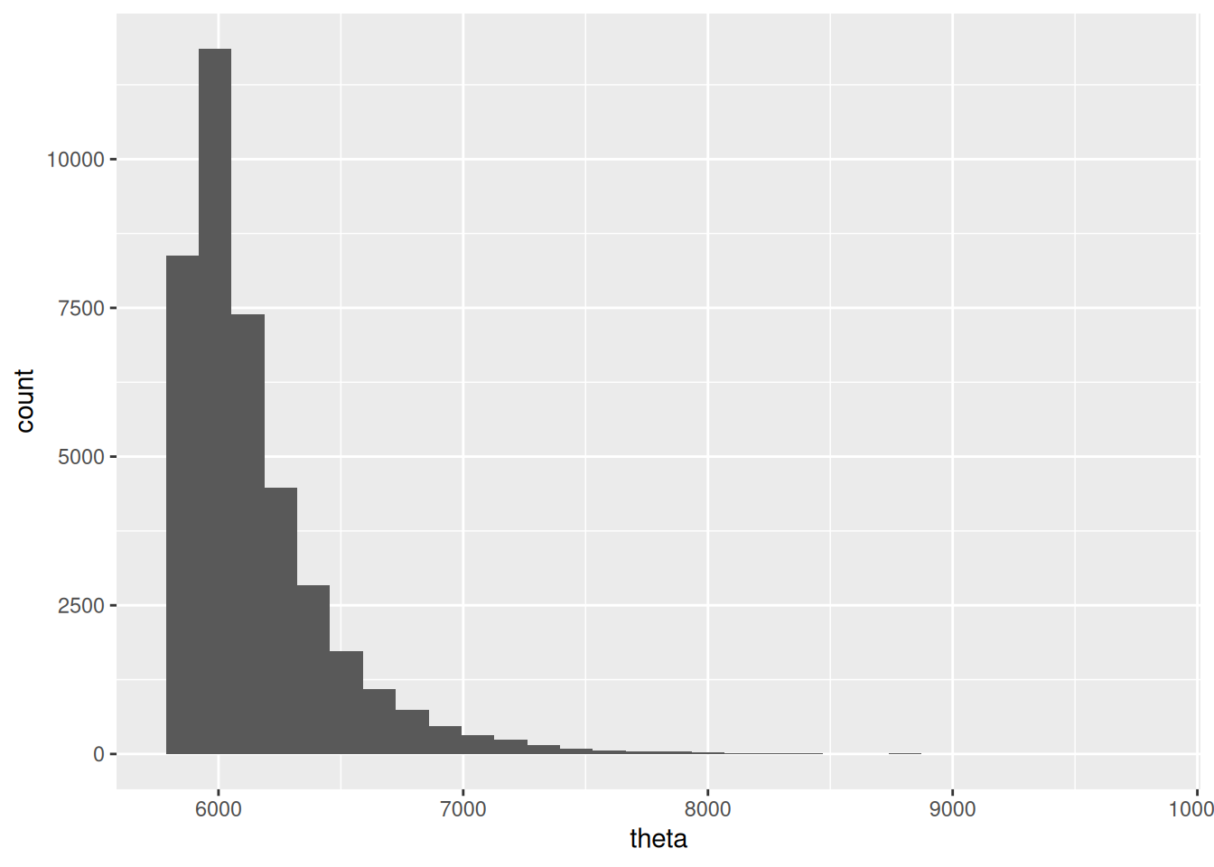
Ejemplo de cantantes
Haremos el ejemplo no conjugado de estaturas de cantantes, con verificación predictiva posterior.
mod## // Ejemplo de modelo normal para estaturas de cantantes
## data {
## int n; // número de observaciones
## array[n] real y; //datos observados
## }
##
## parameters {
## real mu;
## real<lower=2, upper=20> sigma;
## }
##
## model {
## // inicial
## mu ~ normal(175, 3);
## sigma ~ uniform(2, 20);
## y ~ normal(mu, sigma);
## }
##
## generated quantities {
## array[n] real y_sim;
## for(i in 1:n){
## y_sim[i] = normal_rng(mu, sigma);
## }
##
## }Pasamos datos y muestreamos
set.seed(3413)
cantantes <- lattice::singer |>
  mutate(estatura_cm = (2.54 * height)) |>
  filter(str_detect(voice.part, "Tenor")) |>
  sample_n(20)
datos_lista <- list(n = nrow(cantantes), y = cantantes$estatura_cm)
ajuste <- mod$sample(
  data = datos_lista,
  seed = 1234,
  chains = 4,
  iter_warmup = 4000,
  iter_sampling = 4000,
  refresh = 2000)
## Running MCMC with 4 sequential chains...
##
## Chain 1 Iteration: 1 / 8000 [ 0%] (Warmup)
## Chain 1 Iteration: 2000 / 8000 [ 25%] (Warmup)
## Chain 1 Iteration: 4000 / 8000 [ 50%] (Warmup)
## Chain 1 Iteration: 4001 / 8000 [ 50%] (Sampling)
## Chain 1 Iteration: 6000 / 8000 [ 75%] (Sampling)
## Chain 1 Iteration: 8000 / 8000 [100%] (Sampling)
## Chain 1 finished in 0.1 seconds.
## Chain 2 Iteration: 1 / 8000 [ 0%] (Warmup)
## Chain 2 Iteration: 2000 / 8000 [ 25%] (Warmup)
## Chain 2 Iteration: 4000 / 8000 [ 50%] (Warmup)
## Chain 2 Iteration: 4001 / 8000 [ 50%] (Sampling)
## Chain 2 Iteration: 6000 / 8000 [ 75%] (Sampling)
## Chain 2 Iteration: 8000 / 8000 [100%] (Sampling)
## Chain 2 finished in 0.1 seconds.
## Chain 3 Iteration: 1 / 8000 [ 0%] (Warmup)
## Chain 3 Iteration: 2000 / 8000 [ 25%] (Warmup)
## Chain 3 Iteration: 4000 / 8000 [ 50%] (Warmup)
## Chain 3 Iteration: 4001 / 8000 [ 50%] (Sampling)
## Chain 3 Iteration: 6000 / 8000 [ 75%] (Sampling)
## Chain 3 Iteration: 8000 / 8000 [100%] (Sampling)
## Chain 3 finished in 0.1 seconds.
## Chain 4 Iteration: 1 / 8000 [ 0%] (Warmup)
## Chain 4 Iteration: 2000 / 8000 [ 25%] (Warmup)
## Chain 4 Iteration: 4000 / 8000 [ 50%] (Warmup)
## Chain 4 Iteration: 4001 / 8000 [ 50%] (Sampling)
## Chain 4 Iteration: 6000 / 8000 [ 75%] (Sampling)
## Chain 4 Iteration: 8000 / 8000 [100%] (Sampling)
## Chain 4 finished in 0.1 seconds.
##
## All 4 chains finished successfully.
## Mean chain execution time: 0.1 seconds.
## Total execution time: 0.5 seconds.Checamos diagnósticos:
ajuste$cmdstan_diagnose()## Checking sampler transitions treedepth.
## Treedepth satisfactory for all transitions.
##
## Checking sampler transitions for divergences.
## No divergent transitions found.
##
## Checking E-BFMI - sampler transitions HMC potential energy.
## E-BFMI satisfactory.
##
## Rank-normalized split effective sample size satisfactory for all parameters.
##
## Rank-normalized split R-hat values satisfactory for all parameters.
##
## Processing complete, no problems detected.Si no hay problemas, podemos ver el resumen:
resumen <- ajuste$summary()
resumen
## # A tibble: 23 × 10
## variable mean median sd mad q5 q95 rhat ess_bulk ess_tail
## <chr> <dbl> <dbl> <dbl> <dbl> <dbl> <dbl> <dbl> <dbl> <dbl>
## 1 lp__ -46.2 -45.8 1.05 0.753 -48.2 -45.2 1.00 6583. 8196.
## 2 mu 176. 176. 1.33 1.30 174. 178. 1.00 10005. 9087.
## 3 sigma 6.71 6.55 1.18 1.09 5.09 8.86 1.00 9927. 8352.
## 4 y_sim[1] 176. 176. 6.94 6.66 164. 187. 1.00 14414. 15187.
## 5 y_sim[2] 176. 176. 6.98 6.64 164. 187. 1.000 15189. 15317.
## 6 y_sim[3] 176. 176. 6.90 6.60 165. 187. 1.00 15498. 15447.
## 7 y_sim[4] 176. 176. 6.90 6.63 165. 187. 1.00 15421. 15051.
## 8 y_sim[5] 176. 176. 6.89 6.69 165. 187. 1.00 14356. 15532.
## 9 y_sim[6] 176. 176. 6.98 6.67 164. 187. 1.00 15073. 15233.
## 10 y_sim[7] 176. 176. 6.99 6.83 164. 187. 1.00 14656. 15308.
## # ℹ 13 more rowsEl intervalo 95% que obtenemos es:
ajuste$draws(c("mu", "sigma")) |> as_draws_df() |>
ggplot(aes(x = mu, y = sigma)) + geom_point(alpha = 0.1) +
  coord_equal()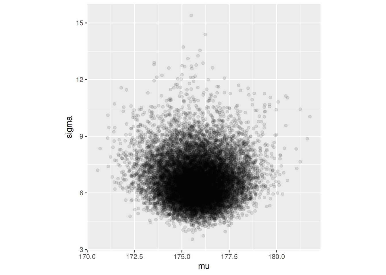
Y ahora extraemos algunas replicaciones de la posterior predictiva:
y_sim_tbl <- ajuste$draws("y_sim") |> as_draws_df() |>
  pivot_longer(cols = starts_with("y_sim")) |>
  filter(.chain == 1, .iteration < 12) |>
  select(.iteration, value) |>
  bind_rows(tibble(.iteration = 12, value = round(cantantes$estatura_cm, 0)))
## Warning: Dropping 'draws_df' class as required metadata was removed.ggplot(y_sim_tbl, aes(sample = value)) +
geom_qq() +
facet_wrap(~ .iteration)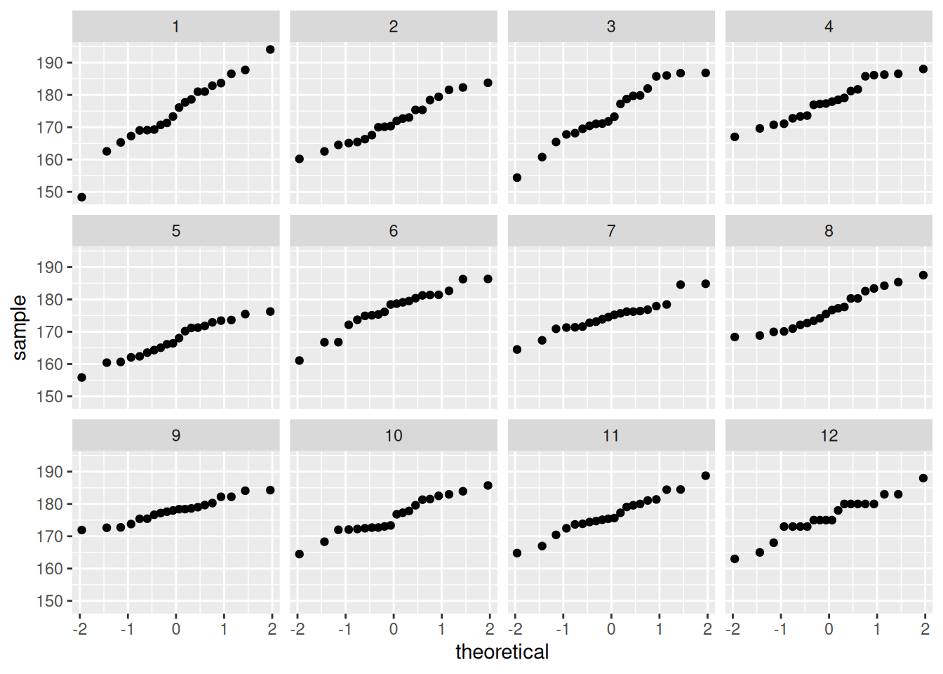
13.0.1 Ejemplo: exámenes
sim_formas <- function(p_azar, p_corr){
  tipo <- rbinom(1, 1, 1 - p_azar)
  if(tipo==0){
    # al azar
    x <- rbinom(1, 10, 1/5)
  } else {
    # no al azar
    x <- rbinom(1, 10, p_corr)
  }
  x
}
set.seed(12)
muestra_1 <- map_dbl(1:200, ~ sim_formas(0.35, 0.5))mod_informado## // Ejemplo de estimación del máximo de uniforme
## data {
## int n; // número de observaciones
## array[n] int y; //datos observados
## }
##
##
## parameters {
## real<lower=0, upper=1> theta_azar;
## real<lower=0, upper=1> theta_corr;
## }
##
## model {
## // inicial
## theta_azar ~ beta(1, 5);
## theta_corr ~ beta(7, 3);
## // en este caso, agregamos términos directamente a la log posterior
## for(i in 1:n){
## target+= log_sum_exp(
## log(theta_azar) + binomial_lpmf(y[i] | 10, 0.20),
## log(1 - theta_azar) + binomial_lpmf(y[i] | 10, theta_corr));
## }
## }Pasamos datos y muestreamos
set.seed(3413)
datos_lista <- list(n = length(muestra_1), y = muestra_1)
ajuste <- mod_informado$sample(
  data = datos_lista,
  seed = 1234,
  chains = 4,
  iter_warmup = 4000,
  iter_sampling = 4000,
  refresh = 2000)
## Running MCMC with 4 sequential chains...
##
## Chain 1 Iteration: 1 / 8000 [ 0%] (Warmup)
## Chain 1 Iteration: 2000 / 8000 [ 25%] (Warmup)
## Chain 1 Iteration: 4000 / 8000 [ 50%] (Warmup)
## Chain 1 Iteration: 4001 / 8000 [ 50%] (Sampling)
## Chain 1 Iteration: 6000 / 8000 [ 75%] (Sampling)
## Chain 1 Iteration: 8000 / 8000 [100%] (Sampling)
## Chain 1 finished in 2.2 seconds.
## Chain 2 Iteration: 1 / 8000 [ 0%] (Warmup)
## Chain 2 Iteration: 2000 / 8000 [ 25%] (Warmup)
## Chain 2 Iteration: 4000 / 8000 [ 50%] (Warmup)
## Chain 2 Iteration: 4001 / 8000 [ 50%] (Sampling)
## Chain 2 Iteration: 6000 / 8000 [ 75%] (Sampling)
## Chain 2 Iteration: 8000 / 8000 [100%] (Sampling)
## Chain 2 finished in 2.1 seconds.
## Chain 3 Iteration: 1 / 8000 [ 0%] (Warmup)
## Chain 3 Iteration: 2000 / 8000 [ 25%] (Warmup)
## Chain 3 Iteration: 4000 / 8000 [ 50%] (Warmup)
## Chain 3 Iteration: 4001 / 8000 [ 50%] (Sampling)
## Chain 3 Iteration: 6000 / 8000 [ 75%] (Sampling)
## Chain 3 Iteration: 8000 / 8000 [100%] (Sampling)
## Chain 3 finished in 2.2 seconds.
## Chain 4 Iteration: 1 / 8000 [ 0%] (Warmup)
## Chain 4 Iteration: 2000 / 8000 [ 25%] (Warmup)
## Chain 4 Iteration: 4000 / 8000 [ 50%] (Warmup)
## Chain 4 Iteration: 4001 / 8000 [ 50%] (Sampling)
## Chain 4 Iteration: 6000 / 8000 [ 75%] (Sampling)
## Chain 4 Iteration: 8000 / 8000 [100%] (Sampling)
## Chain 4 finished in 2.0 seconds.
##
## All 4 chains finished successfully.
## Mean chain execution time: 2.1 seconds.
## Total execution time: 8.8 seconds.Checamos diagnósticos:
ajuste$cmdstan_diagnose()## Checking sampler transitions treedepth.
## Treedepth satisfactory for all transitions.
##
## Checking sampler transitions for divergences.
## No divergent transitions found.
##
## Checking E-BFMI - sampler transitions HMC potential energy.
## E-BFMI satisfactory.
##
## Rank-normalized split effective sample size satisfactory for all parameters.
##
## Rank-normalized split R-hat values satisfactory for all parameters.
##
## Processing complete, no problems detected.Si no hay problemas, podemos ver el resumen:
resumen <- ajuste$summary()
resumen
## # A tibble: 3 × 10
## variable mean median sd mad q5 q95 rhat ess_bulk
## <chr> <dbl> <dbl> <dbl> <dbl> <dbl> <dbl> <dbl> <dbl>
## 1 lp__ -439. -438. 1.02 0.712 -441. -438. 1.00 7491.
## 2 theta_azar 0.373 0.372 0.0466 0.0469 0.297 0.449 1.000 7682.
## 3 theta_corr 0.524 0.524 0.0183 0.0182 0.494 0.555 1.00 7828.
## # ℹ 1 more variable: ess_tail <dbl>sims_theta_tbl <-
ajuste$draws(c("theta_azar", "theta_corr")) |>
as_draws_df()
ggplot(sims_theta_tbl, aes(x = theta_azar, y = theta_corr)) +
geom_point(alpha = 0.1)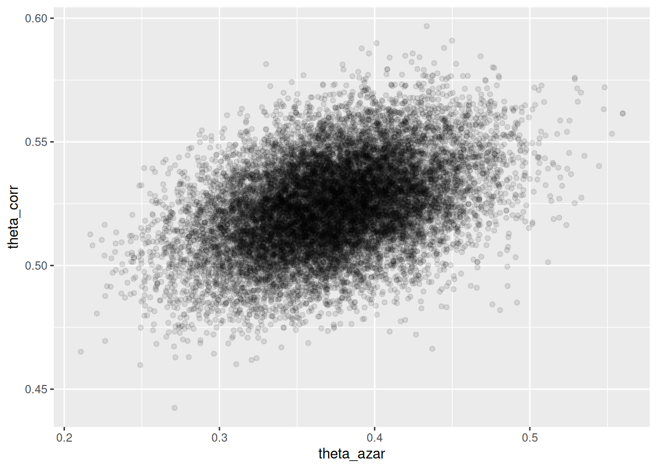
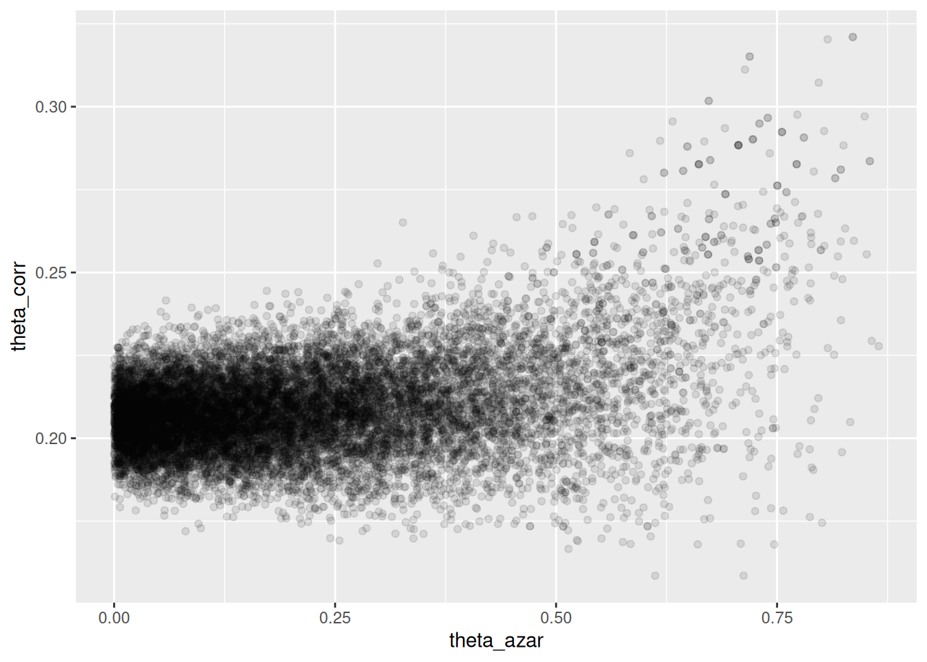
13.1 Ejemplo: exámenes, mal identificado
En este ejemplo cambiamos los parámetros de la simulación y ponemos iniciales poco informativas.
set.seed(12)
muestra_2 <- map_dbl(1:200, ~ sim_formas(0.35, 0.21))mod_no_inf## // Ejemplo de estimación del máximo de uniforme
## data {
## int n; // número de observaciones
## array[n] int y; //datos observados
## }
##
##
## parameters {
## real<lower=0, upper=1> theta_azar;
## real<lower=0, upper=1> theta_corr;
## }
##
## model {
## // inicial
## theta_azar ~ beta(1, 1);
## theta_corr ~ beta(1, 1);
## // en este caso, agregamos términos directamente a la log posterior
## for(i in 1:n){
## target+= log_sum_exp(
## log(theta_azar) + binomial_lpmf(y[i] | 10, 0.20),
## log(1 - theta_azar) + binomial_lpmf(y[i] | 10, theta_corr));
## }
## }Pasamos datos y muestreamos
set.seed(3413)
datos_lista <- list(n = length(muestra_2), y = muestra_2)
ajuste <- mod_no_inf$sample(
data = datos_lista,
seed = 1234,
chains = 4,
iter_warmup = 4000,
iter_sampling = 4000,
refresh = 2000)## Running MCMC with 4 sequential chains...
##
## Chain 1 Iteration: 1 / 8000 [ 0%] (Warmup)
## Chain 1 Iteration: 2000 / 8000 [ 25%] (Warmup)
## Chain 1 Iteration: 4000 / 8000 [ 50%] (Warmup)
## Chain 1 Iteration: 4001 / 8000 [ 50%] (Sampling)
## Chain 1 Iteration: 6000 / 8000 [ 75%] (Sampling)
## Chain 1 Iteration: 8000 / 8000 [100%] (Sampling)
## Chain 1 finished in 3.3 seconds.
## Chain 2 Iteration: 1 / 8000 [ 0%] (Warmup)
## Chain 2 Iteration: 2000 / 8000 [ 25%] (Warmup)
## Chain 2 Iteration: 4000 / 8000 [ 50%] (Warmup)
## Chain 2 Iteration: 4001 / 8000 [ 50%] (Sampling)
## Chain 2 Iteration: 6000 / 8000 [ 75%] (Sampling)
## Chain 2 Iteration: 8000 / 8000 [100%] (Sampling)
## Chain 2 finished in 3.1 seconds.
## Chain 3 Iteration: 1 / 8000 [ 0%] (Warmup)
## Chain 3 Iteration: 2000 / 8000 [ 25%] (Warmup)
## Chain 3 Iteration: 4000 / 8000 [ 50%] (Warmup)
## Chain 3 Iteration: 4001 / 8000 [ 50%] (Sampling)
## Chain 3 Iteration: 6000 / 8000 [ 75%] (Sampling)
## Chain 3 Iteration: 8000 / 8000 [100%] (Sampling)
## Chain 3 finished in 3.4 seconds.
## Chain 4 Iteration: 1 / 8000 [ 0%] (Warmup)
## Chain 4 Iteration: 2000 / 8000 [ 25%] (Warmup)
## Chain 4 Iteration: 4000 / 8000 [ 50%] (Warmup)
## Chain 4 Iteration: 4001 / 8000 [ 50%] (Sampling)
## Chain 4 Iteration: 6000 / 8000 [ 75%] (Sampling)
## Chain 4 Iteration: 8000 / 8000 [100%] (Sampling)
## Chain 4 finished in 3.2 seconds.
##
## All 4 chains finished successfully.
## Mean chain execution time: 3.3 seconds.
## Total execution time: 13.2 seconds.## Warning: 196 of 16000 (1.0%) transitions ended with a divergence.
## See https://mc-stan.org/misc/warnings for details.Y obtenemos mensajes de advertencia (divergencias), lo que implica que los diagnósticos indican que es posible que las cadenas no hayan explorado suficientemente la posterior
ajuste$cmdstan_diagnose()## Checking sampler transitions treedepth.
## Treedepth satisfactory for all transitions.
##
## Checking sampler transitions for divergences.
## 196 of 16000 (1.23%) transitions ended with a divergence.
## These divergent transitions indicate that HMC is not fully able to explore the posterior distribution.
## Try increasing adapt delta closer to 1.
## If this doesn't remove all divergences, try to reparameterize the model.
##
## Checking E-BFMI - sampler transitions HMC potential energy.
## E-BFMI satisfactory.
##
## Rank-normalized split effective sample size satisfactory for all parameters.
##
## Rank-normalized split R-hat values satisfactory for all parameters.
##
## Processing complete.sims_theta_tbl <-
ajuste$draws(c("theta_azar", "theta_corr")) |>
as_draws_df()
ggplot(sims_theta_tbl, aes(x = theta_azar, y = theta_corr)) +
geom_point(alpha = 0.1)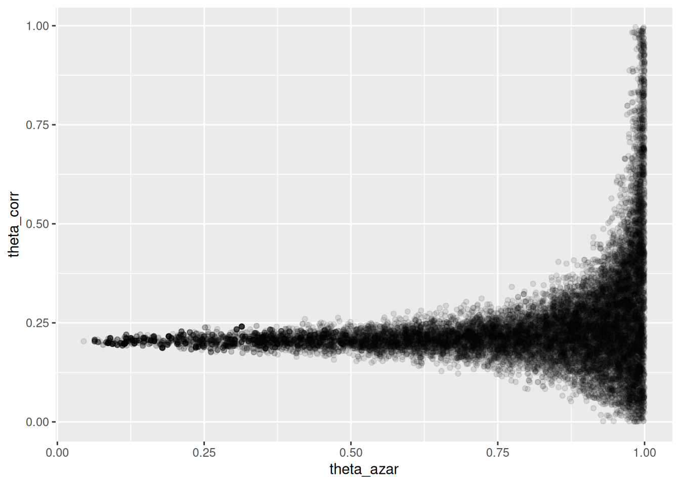
Donde vemos que el problema es serio: cuando \(\theta_{azar}\) es chico, los datos son consistentes con valores de \(\theta_{corr}\) cercanos a 0.2. Pero también es posible que \(\theta_{azar}\) sea grande, y en ese caso tenemos poca información acerca de \(\theta_corr\).
- La geometría de esta posterior hace difícil para el algoritmo establecer el tamaño de paso correcto para explorar adecuadamente esta posterior (con un tamaño de paso chico, explora lentamente, pero si se hace más grande, entonces aparecen problemas numéricos y rechazos en los “embudos” de esta posterior).
- Sin embargo, este resultado generalmente lo rechazaríamos, pues sabemos que una proporción considerable de estudiantes no contesta al azar.
Si corremos el modelo informado con la muestra de esta población, obtenemos:
set.seed(3413)
datos_lista <- list(n = length(muestra_2), y = muestra_2)
ajuste <- mod_informado$sample(
data = datos_lista,
seed = 1234,
chains = 4,
iter_warmup = 4000,
iter_sampling = 4000,
refresh = 2000)## Running MCMC with 4 sequential chains...
##
## Chain 1 Iteration: 1 / 8000 [ 0%] (Warmup)
## Chain 1 Iteration: 2000 / 8000 [ 25%] (Warmup)
## Chain 1 Iteration: 4000 / 8000 [ 50%] (Warmup)
## Chain 1 Iteration: 4001 / 8000 [ 50%] (Sampling)
## Chain 1 Iteration: 6000 / 8000 [ 75%] (Sampling)
## Chain 1 Iteration: 8000 / 8000 [100%] (Sampling)
## Chain 1 finished in 2.0 seconds.
## Chain 2 Iteration: 1 / 8000 [ 0%] (Warmup)
## Chain 2 Iteration: 2000 / 8000 [ 25%] (Warmup)
## Chain 2 Iteration: 4000 / 8000 [ 50%] (Warmup)
## Chain 2 Iteration: 4001 / 8000 [ 50%] (Sampling)
## Chain 2 Iteration: 6000 / 8000 [ 75%] (Sampling)
## Chain 2 Iteration: 8000 / 8000 [100%] (Sampling)
## Chain 2 finished in 2.0 seconds.
## Chain 3 Iteration: 1 / 8000 [ 0%] (Warmup)
## Chain 3 Iteration: 2000 / 8000 [ 25%] (Warmup)
## Chain 3 Iteration: 4000 / 8000 [ 50%] (Warmup)
## Chain 3 Iteration: 4001 / 8000 [ 50%] (Sampling)
## Chain 3 Iteration: 6000 / 8000 [ 75%] (Sampling)
## Chain 3 Iteration: 8000 / 8000 [100%] (Sampling)
## Chain 3 finished in 2.2 seconds.
## Chain 4 Iteration: 1 / 8000 [ 0%] (Warmup)
## Chain 4 Iteration: 2000 / 8000 [ 25%] (Warmup)
## Chain 4 Iteration: 4000 / 8000 [ 50%] (Warmup)
## Chain 4 Iteration: 4001 / 8000 [ 50%] (Sampling)
## Chain 4 Iteration: 6000 / 8000 [ 75%] (Sampling)
## Chain 4 Iteration: 8000 / 8000 [100%] (Sampling)
## Chain 4 finished in 2.1 seconds.
##
## All 4 chains finished successfully.
## Mean chain execution time: 2.1 seconds.
## Total execution time: 8.7 seconds.No tenemos problemas numéricos, y la posterior se ve como sigue:
sims_theta_tbl <-
  ajuste$draws(c("theta_azar", "theta_corr")) |>
  as_draws_df()
ggplot(sims_theta_tbl, aes(x = theta_azar, y = theta_corr)) +
  geom_point(alpha = 0.1)