Sección 13 Ejemplos de inferencia bayesiana en Stan I
En esta parte veremos cómo correr y diagnosticar en Stan varios ejemplos vistos en clase. Para instalar cmdstanr y Stan, puedes ver aquí. En python puedes usar pystan, por ejemplo.
# install.packages("cmdstanr", repos = c("https://mc-stan.org/r-packages/", getOption("repos")))
library(cmdstanr)
library(posterior)
library(tidyverse)
Estimación de una proporción
Escribimos el código para el modelo en un archivo modelo-1.stan, y compilamos:
archivo_stan <- file.path("stan/modelo-1.stan")
# compilar
mod <- cmdstan_model(archivo_stan)mod## // Ejemplo de estimación de una proporcion
## data {
## int n; // número de pruebas
## int y; //numero de éxitos y fracasos
## }
##
## parameters {
## real<lower=0,upper=1> theta;
## }
##
## model {
## // inicial
## theta ~ beta(3, 3);
## y ~ binomial(n, theta);
## }
##
## generated quantities {
## real theta_inicial;
## theta_inicial = beta_rng(3, 3);
## }Pasamos datos y muestreamos
datos_lista <- list(n = 30, y = 19)
ajuste <- mod$sample(
  data = datos_lista,
  seed = 1234,
  chains = 4,
  parallel_chains = 4,
  refresh = 500)
## Running MCMC with 4 parallel chains...
##
## Chain 1 Iteration: 1 / 2000 [ 0%] (Warmup)
## Chain 1 Iteration: 500 / 2000 [ 25%] (Warmup)
## Chain 1 Iteration: 1000 / 2000 [ 50%] (Warmup)
## Chain 1 Iteration: 1001 / 2000 [ 50%] (Sampling)
## Chain 1 Iteration: 1500 / 2000 [ 75%] (Sampling)
## Chain 1 Iteration: 2000 / 2000 [100%] (Sampling)
## Chain 2 Iteration: 1 / 2000 [ 0%] (Warmup)
## Chain 2 Iteration: 500 / 2000 [ 25%] (Warmup)
## Chain 2 Iteration: 1000 / 2000 [ 50%] (Warmup)
## Chain 2 Iteration: 1001 / 2000 [ 50%] (Sampling)
## Chain 2 Iteration: 1500 / 2000 [ 75%] (Sampling)
## Chain 2 Iteration: 2000 / 2000 [100%] (Sampling)
## Chain 3 Iteration: 1 / 2000 [ 0%] (Warmup)
## Chain 3 Iteration: 500 / 2000 [ 25%] (Warmup)
## Chain 3 Iteration: 1000 / 2000 [ 50%] (Warmup)
## Chain 3 Iteration: 1001 / 2000 [ 50%] (Sampling)
## Chain 3 Iteration: 1500 / 2000 [ 75%] (Sampling)
## Chain 3 Iteration: 2000 / 2000 [100%] (Sampling)
## Chain 4 Iteration: 1 / 2000 [ 0%] (Warmup)
## Chain 4 Iteration: 500 / 2000 [ 25%] (Warmup)
## Chain 4 Iteration: 1000 / 2000 [ 50%] (Warmup)
## Chain 4 Iteration: 1001 / 2000 [ 50%] (Sampling)
## Chain 4 Iteration: 1500 / 2000 [ 75%] (Sampling)
## Chain 4 Iteration: 2000 / 2000 [100%] (Sampling)
## Chain 1 finished in 0.0 seconds.
## Chain 2 finished in 0.0 seconds.
## Chain 3 finished in 0.0 seconds.
## Chain 4 finished in 0.0 seconds.
##
## All 4 chains finished successfully.
## Mean chain execution time: 0.0 seconds.
## Total execution time: 0.3 seconds.Checamos diagnósticos:
ajuste$cmdstan_diagnose()## Processing csv files: /tmp/Rtmpv7c8tl/modelo-1-202311292012-1-8a4b85.csv, /tmp/Rtmpv7c8tl/modelo-1-202311292012-2-8a4b85.csv, /tmp/Rtmpv7c8tl/modelo-1-202311292012-3-8a4b85.csv, /tmp/Rtmpv7c8tl/modelo-1-202311292012-4-8a4b85.csv
##
## Checking sampler transitions treedepth.
## Treedepth satisfactory for all transitions.
##
## Checking sampler transitions for divergences.
## No divergent transitions found.
##
## Checking E-BFMI - sampler transitions HMC potential energy.
## E-BFMI satisfactory.
##
## Effective sample size satisfactory.
##
## Split R-hat values satisfactory all parameters.
##
## Processing complete, no problems detected.Si no hay problemas, podemos ver el resumen:
ajuste$summary()## # A tibble: 3 × 10
## variable mean median sd mad q5 q95 rhat ess_bulk ess_tail
## <chr> <num> <num> <num> <num> <num> <num> <num> <num> <num>
## 1 lp__ -24.5 -24.3 0.694 0.289 -26.0 -24.1 1.00 1845. 2051.
## 2 theta 0.611 0.613 0.0787 0.0786 0.476 0.739 1.00 1324. 1635.
## 3 theta_i… 0.500 0.502 0.190 0.208 0.189 0.813 1.00 4182. 4102.Donde verificamos que el tamaño de muestra efectivo (ess) y el diagnóstico de \(\hat{R}\) son apropiados.
Podemos ver las cadenas de la siguiente forma:
theta_tbl <- ajuste$draws(c("theta", "theta_inicial")) %>% as_draws_df()
ggplot(theta_tbl, aes(x = .iteration, y = theta)) +
  geom_line() +
  facet_wrap(~.chain, ncol = 1)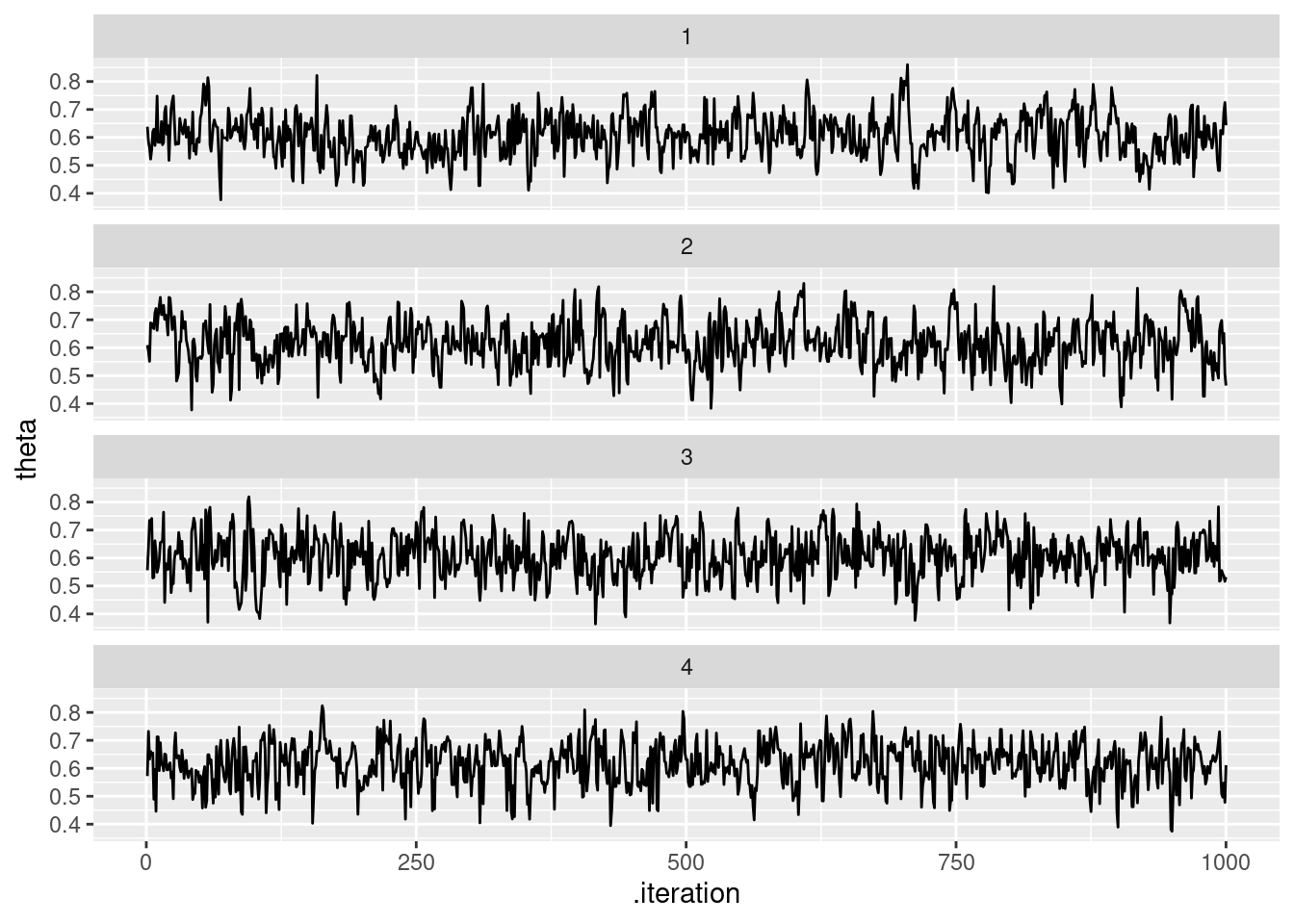
Y replicamos la gráfica de las notas haciendo:
sims_tbl <- theta_tbl %>% pivot_longer(theta:theta_inicial, names_to = "dist", values_to = "theta")## Warning: Dropping 'draws_df' class as required metadata was removed.ggplot(sims_tbl, aes(x = theta, fill = dist)) +
geom_histogram(aes(x = theta), bins = 30, alpha = 0.5, position = "identity")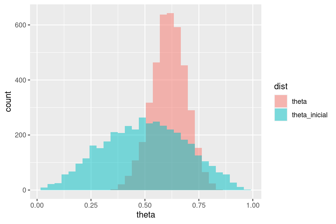
Estimación del máximo de una uniforme
Tomamos el ejemplo de los boletos de lotería,
loteria_tbl <- read_csv("data/nums_loteria_avion.csv", col_names = c("id", "numero")) %>%
  mutate(numero = as.integer(numero))
## Rows: 99 Columns: 2
## ── Column specification ────────────────────────────────────────────────────────
## Delimiter: ","
## chr (1): numero
## dbl (1): id
##
## ℹ Use `spec()` to retrieve the full column specification for this data.
## ℹ Specify the column types or set `show_col_types = FALSE` to quiet this message.set.seed(334)
muestra_loteria <- sample_n(loteria_tbl, 25) %>%
mutate(numero = numero/1000)mod## // Ejemplo de estimación del máximo de uniforme
## data {
## int n; // número de observaciones
## array[n] real y; //datos observados
## }
##
## transformed data{
## real y_max;
## y_max = max(y);
## }
## parameters {
## real<lower=y_max> theta;
## }
##
## model {
## // inicial
## theta ~ pareto(300, 1.1);
## y ~ uniform(0, theta);
## }Pasamos datos y muestreamos:
datos_lista <- list(n = nrow(muestra_loteria), y = muestra_loteria$numero)
ajuste <- mod$sample(
  data = datos_lista,
  seed = 1234,
  chains = 4,
  iter_warmup = 5000,
  iter_sampling = 20000,
  parallel_chains = 4,
  refresh = 5000)
## Running MCMC with 4 parallel chains...
##
## Chain 1 Iteration: 1 / 25000 [ 0%] (Warmup)
## Chain 1 Iteration: 5000 / 25000 [ 20%] (Warmup)
## Chain 1 Iteration: 5001 / 25000 [ 20%] (Sampling)
## Chain 1 Iteration: 10000 / 25000 [ 40%] (Sampling)
## Chain 2 Iteration: 1 / 25000 [ 0%] (Warmup)
## Chain 2 Iteration: 5000 / 25000 [ 20%] (Warmup)
## Chain 2 Iteration: 5001 / 25000 [ 20%] (Sampling)
## Chain 2 Iteration: 10000 / 25000 [ 40%] (Sampling)
## Chain 3 Iteration: 1 / 25000 [ 0%] (Warmup)
## Chain 3 Iteration: 5000 / 25000 [ 20%] (Warmup)
## Chain 3 Iteration: 5001 / 25000 [ 20%] (Sampling)
## Chain 3 Iteration: 10000 / 25000 [ 40%] (Sampling)## Chain 3 Informational Message: The current Metropolis proposal is about to be rejected because of the following issue:## Chain 3 Exception: uniform_lpdf: Upper bound parameter is inf, but must be finite! (in '/tmp/Rtmpv7c8tl/model-26ca41633101.stan', line 18, column 2 to column 24)## Chain 3 If this warning occurs sporadically, such as for highly constrained variable types like covariance matrices, then the sampler is fine,## Chain 3 but if this warning occurs often then your model may be either severely ill-conditioned or misspecified.## Chain 3## Chain 4 Iteration: 1 / 25000 [ 0%] (Warmup)
## Chain 4 Iteration: 5000 / 25000 [ 20%] (Warmup)
## Chain 4 Iteration: 5001 / 25000 [ 20%] (Sampling)
## Chain 4 Iteration: 10000 / 25000 [ 40%] (Sampling)
## Chain 1 Iteration: 15000 / 25000 [ 60%] (Sampling)
## Chain 1 Iteration: 20000 / 25000 [ 80%] (Sampling)
## Chain 1 Iteration: 25000 / 25000 [100%] (Sampling)
## Chain 2 Iteration: 15000 / 25000 [ 60%] (Sampling)
## Chain 2 Iteration: 20000 / 25000 [ 80%] (Sampling)
## Chain 3 Iteration: 15000 / 25000 [ 60%] (Sampling)
## Chain 3 Iteration: 20000 / 25000 [ 80%] (Sampling)
## Chain 3 Iteration: 25000 / 25000 [100%] (Sampling)
## Chain 4 Iteration: 15000 / 25000 [ 60%] (Sampling)
## Chain 1 finished in 0.3 seconds.
## Chain 2 Iteration: 25000 / 25000 [100%] (Sampling)
## Chain 2 finished in 0.3 seconds.
## Chain 3 finished in 0.3 seconds.
## Chain 4 Iteration: 20000 / 25000 [ 80%] (Sampling)
## Chain 4 Iteration: 25000 / 25000 [100%] (Sampling)
## Chain 4 finished in 0.3 seconds.
##
## All 4 chains finished successfully.
## Mean chain execution time: 0.3 seconds.
## Total execution time: 0.5 seconds.Checamos diagnósticos:
ajuste$cmdstan_diagnose()## Processing csv files: /tmp/Rtmpv7c8tl/modelo-2-202311292012-1-7abdbd.csv, /tmp/Rtmpv7c8tl/modelo-2-202311292012-2-7abdbd.csv, /tmp/Rtmpv7c8tl/modelo-2-202311292012-3-7abdbd.csv, /tmp/Rtmpv7c8tl/modelo-2-202311292012-4-7abdbd.csv
##
## Checking sampler transitions treedepth.
## Treedepth satisfactory for all transitions.
##
## Checking sampler transitions for divergences.
## No divergent transitions found.
##
## Checking E-BFMI - sampler transitions HMC potential energy.
## E-BFMI satisfactory.
##
## Effective sample size satisfactory.
##
## Split R-hat values satisfactory all parameters.
##
## Processing complete, no problems detected.Si no hay problemas, podemos ver el resumen:
resumen <- ajuste$summary()
resumen
## # A tibble: 2 × 10
## variable mean median sd mad q5 q95 rhat ess_bulk ess_tail
## <chr> <num> <num> <num> <num> <num> <num> <num> <num> <num>
## 1 lp__ -231. -231. 0.793 0.359 -233. -231. 1.00 23508. 21069.
## 2 theta 6087. 6012. 243. 165. 5864. 6567. 1.00 20929. 18821.El intervalo 95% que obtenemos es:
ajuste$draws("theta") %>% as_draws_df() %>%
  summarise(theta_inf = quantile(theta, 0.025),
            theta_mediana = quantile(theta, 0.5),
            theta_sup = quantile(theta, 0.975))
## # A tibble: 1 × 3
## theta_inf theta_mediana theta_sup
## <dbl> <dbl> <dbl>
## 1 5858. 6012. 6742.Podemos ahora intentar con la inicial gamma que nos pareció más intuitiva, aún cuando el modelo no es conjugado:
archivo_stan <- file.path("stan/modelo-3.stan")
# compilar
mod <- cmdstan_model(archivo_stan)mod## // Ejemplo de estimación del máximo de uniforme
## data {
## int n; // número de observaciones
## array[n] real y; //datos observados
## }
##
## transformed data{
## real y_max;
## y_max = max(y);
## }
## parameters {
## real<lower=y_max> theta;
## }
##
## model {
## // inicial
## theta ~ gamma(5, 0.0001);
## y ~ uniform(0, theta);
## }Pasamos datos y muestreamos
datos_lista <- list(n = nrow(muestra_loteria), y = muestra_loteria$numero)
ajuste <- mod$sample(
  data = datos_lista,
  seed = 1234,
  chains = 4,
  iter_sampling = 10000,
  parallel_chains = 4,
  refresh = 2000)
## Running MCMC with 4 parallel chains...
##
## Chain 1 Iteration: 1 / 11000 [ 0%] (Warmup)
## Chain 1 Iteration: 1001 / 11000 [ 9%] (Sampling)
## Chain 1 Iteration: 3000 / 11000 [ 27%] (Sampling)
## Chain 1 Iteration: 5000 / 11000 [ 45%] (Sampling)
## Chain 1 Iteration: 7000 / 11000 [ 63%] (Sampling)
## Chain 1 Iteration: 9000 / 11000 [ 81%] (Sampling)
## Chain 1 Iteration: 11000 / 11000 [100%] (Sampling)
## Chain 2 Iteration: 1 / 11000 [ 0%] (Warmup)
## Chain 2 Iteration: 1001 / 11000 [ 9%] (Sampling)
## Chain 2 Iteration: 3000 / 11000 [ 27%] (Sampling)
## Chain 2 Iteration: 5000 / 11000 [ 45%] (Sampling)
## Chain 2 Iteration: 7000 / 11000 [ 63%] (Sampling)
## Chain 2 Iteration: 9000 / 11000 [ 81%] (Sampling)
## Chain 3 Iteration: 1 / 11000 [ 0%] (Warmup)
## Chain 3 Iteration: 1001 / 11000 [ 9%] (Sampling)
## Chain 3 Iteration: 3000 / 11000 [ 27%] (Sampling)
## Chain 3 Iteration: 5000 / 11000 [ 45%] (Sampling)
## Chain 3 Iteration: 7000 / 11000 [ 63%] (Sampling)
## Chain 3 Iteration: 9000 / 11000 [ 81%] (Sampling)
## Chain 4 Iteration: 1 / 11000 [ 0%] (Warmup)
## Chain 4 Iteration: 1001 / 11000 [ 9%] (Sampling)
## Chain 4 Iteration: 3000 / 11000 [ 27%] (Sampling)
## Chain 4 Iteration: 5000 / 11000 [ 45%] (Sampling)
## Chain 4 Iteration: 7000 / 11000 [ 63%] (Sampling)
## Chain 4 Iteration: 9000 / 11000 [ 81%] (Sampling)
## Chain 1 finished in 0.1 seconds.
## Chain 2 Iteration: 11000 / 11000 [100%] (Sampling)
## Chain 2 finished in 0.1 seconds.
## Chain 3 Iteration: 11000 / 11000 [100%] (Sampling)
## Chain 3 finished in 0.1 seconds.
## Chain 4 Iteration: 11000 / 11000 [100%] (Sampling)
## Chain 4 finished in 0.1 seconds.
##
## All 4 chains finished successfully.
## Mean chain execution time: 0.1 seconds.
## Total execution time: 0.3 seconds.Checamos diagnósticos:
ajuste$cmdstan_diagnose()## Processing csv files: /tmp/Rtmpv7c8tl/modelo-3-202311292012-1-348f41.csv, /tmp/Rtmpv7c8tl/modelo-3-202311292012-2-348f41.csv, /tmp/Rtmpv7c8tl/modelo-3-202311292012-3-348f41.csv, /tmp/Rtmpv7c8tl/modelo-3-202311292012-4-348f41.csv
##
## Checking sampler transitions treedepth.
## Treedepth satisfactory for all transitions.
##
## Checking sampler transitions for divergences.
## No divergent transitions found.
##
## Checking E-BFMI - sampler transitions HMC potential energy.
## E-BFMI satisfactory.
##
## Effective sample size satisfactory.
##
## Split R-hat values satisfactory all parameters.
##
## Processing complete, no problems detected.Si no hay problemas, podemos ver el resumen:
resumen <- ajuste$summary()
resumen
## # A tibble: 2 × 10
## variable mean median sd mad q5 q95 rhat ess_bulk ess_tail
## <chr> <num> <num> <num> <num> <num> <num> <num> <num> <num>
## 1 lp__ -179. -178. 0.799 0.362 -180. -178. 1.00 11507. 10915.
## 2 theta 6150. 6052. 314. 208. 5867. 6764. 1.00 9946. 9364.El intervalo 95% que obtenemos es:
ajuste$draws("theta") %>% as_draws_df() %>%
  summarise(theta_inf = quantile(theta, 0.025),
            theta_mediana = quantile(theta, 0.5),
            theta_sup = quantile(theta, 0.975))
## # A tibble: 1 × 3
## theta_inf theta_mediana theta_sup
## <dbl> <dbl> <dbl>
## 1 5860. 6052. 6996.Y la posterior se ve como sigue:
theta_post_sim <- ajuste$draws("theta") %>% as.numeric
qplot(theta_post_sim)
## Warning: `qplot()` was deprecated in ggplot2 3.4.0.
## This warning is displayed once every 8 hours.
## Call `lifecycle::last_lifecycle_warnings()` to see where this warning was
## generated.## `stat_bin()` using `bins = 30`. Pick better value with `binwidth`.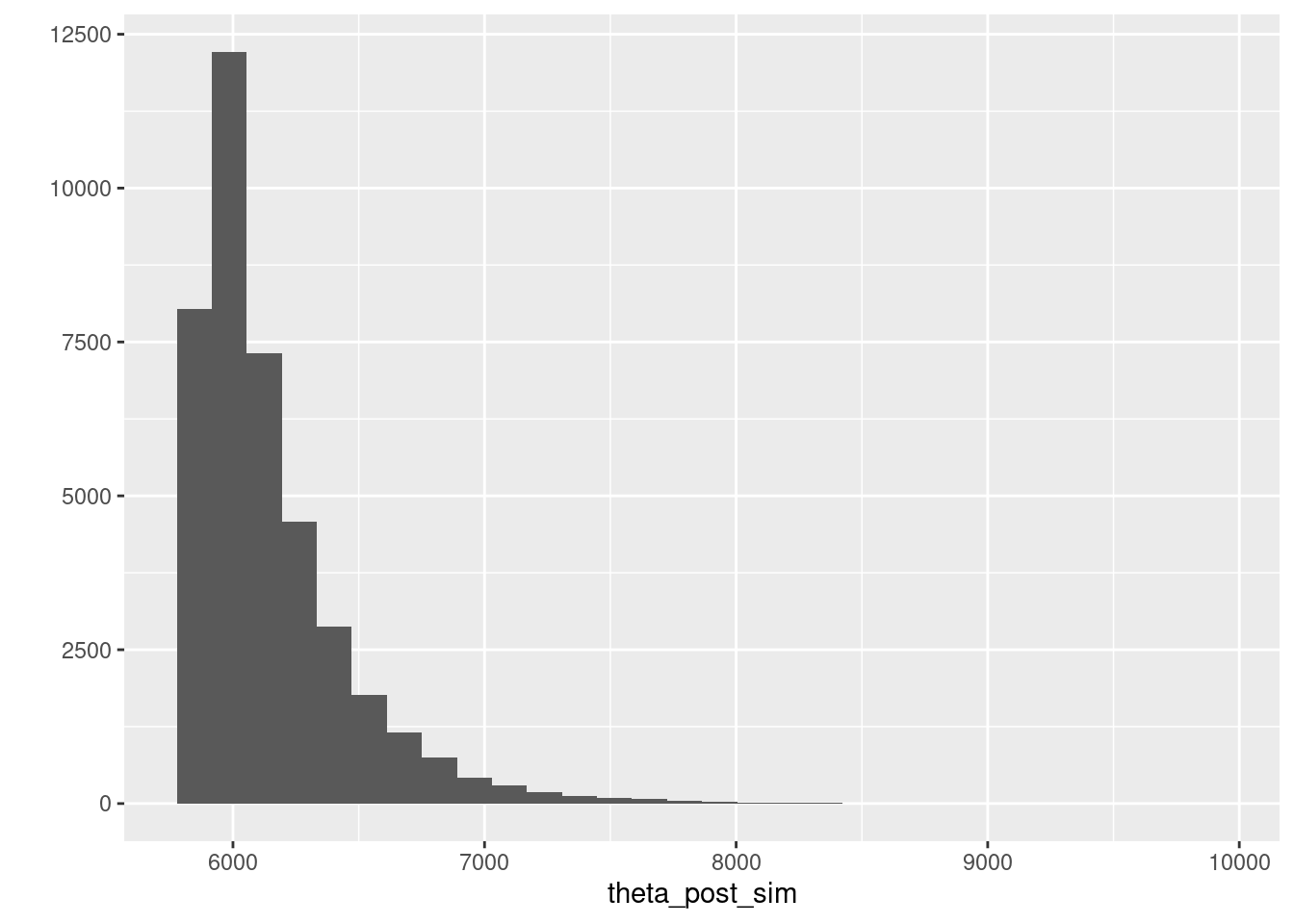
Ejemplo de cantantes
Haremos el ejemplo no conjugado de estaturas de cantantes, con verificación predictiva posterior.
mod## // Ejemplo de modelo normal para estaturas de cantantes
## data {
## int n; // número de observaciones
## array[n] real y; //datos observados
## }
##
## parameters {
## real mu;
## real<lower=2, upper=20> sigma;
## }
##
## model {
## // inicial
## mu ~ normal(175, 3);
## sigma ~ uniform(2, 20);
## y ~ normal(mu, sigma);
## }
##
## generated quantities {
## array[n] real y_sim;
## for(i in 1:n){
## y_sim[i] = normal_rng(mu, sigma);
## }
##
## }Pasamos datos y muestreamos
set.seed(3413)
cantantes <- lattice::singer %>%
  mutate(estatura_cm = (2.54 * height)) %>%
  filter(str_detect(voice.part, "Tenor")) %>%
  sample_n(20)
datos_lista <- list(n = nrow(cantantes), y = cantantes$estatura_cm)
ajuste <- mod$sample(
  data = datos_lista,
  seed = 1234,
  chains = 4,
  iter_warmup = 4000,
  iter_sampling = 4000,
  refresh = 2000)
## Running MCMC with 4 sequential chains...
##
## Chain 1 Iteration: 1 / 8000 [ 0%] (Warmup)
## Chain 1 Iteration: 2000 / 8000 [ 25%] (Warmup)
## Chain 1 Iteration: 4000 / 8000 [ 50%] (Warmup)
## Chain 1 Iteration: 4001 / 8000 [ 50%] (Sampling)
## Chain 1 Iteration: 6000 / 8000 [ 75%] (Sampling)
## Chain 1 Iteration: 8000 / 8000 [100%] (Sampling)
## Chain 1 finished in 0.1 seconds.
## Chain 2 Iteration: 1 / 8000 [ 0%] (Warmup)
## Chain 2 Iteration: 2000 / 8000 [ 25%] (Warmup)
## Chain 2 Iteration: 4000 / 8000 [ 50%] (Warmup)
## Chain 2 Iteration: 4001 / 8000 [ 50%] (Sampling)
## Chain 2 Iteration: 6000 / 8000 [ 75%] (Sampling)
## Chain 2 Iteration: 8000 / 8000 [100%] (Sampling)
## Chain 2 finished in 0.1 seconds.
## Chain 3 Iteration: 1 / 8000 [ 0%] (Warmup)
## Chain 3 Iteration: 2000 / 8000 [ 25%] (Warmup)
## Chain 3 Iteration: 4000 / 8000 [ 50%] (Warmup)
## Chain 3 Iteration: 4001 / 8000 [ 50%] (Sampling)
## Chain 3 Iteration: 6000 / 8000 [ 75%] (Sampling)
## Chain 3 Iteration: 8000 / 8000 [100%] (Sampling)
## Chain 3 finished in 0.1 seconds.
## Chain 4 Iteration: 1 / 8000 [ 0%] (Warmup)
## Chain 4 Iteration: 2000 / 8000 [ 25%] (Warmup)
## Chain 4 Iteration: 4000 / 8000 [ 50%] (Warmup)
## Chain 4 Iteration: 4001 / 8000 [ 50%] (Sampling)
## Chain 4 Iteration: 6000 / 8000 [ 75%] (Sampling)
## Chain 4 Iteration: 8000 / 8000 [100%] (Sampling)
## Chain 4 finished in 0.1 seconds.
##
## All 4 chains finished successfully.
## Mean chain execution time: 0.1 seconds.
## Total execution time: 0.6 seconds.Checamos diagnósticos:
ajuste$cmdstan_diagnose()## Processing csv files: /tmp/Rtmpv7c8tl/modelo-cantantes-202311292013-1-1106ec.csv, /tmp/Rtmpv7c8tl/modelo-cantantes-202311292013-2-1106ec.csv, /tmp/Rtmpv7c8tl/modelo-cantantes-202311292013-3-1106ec.csv, /tmp/Rtmpv7c8tl/modelo-cantantes-202311292013-4-1106ec.csv
##
## Checking sampler transitions treedepth.
## Treedepth satisfactory for all transitions.
##
## Checking sampler transitions for divergences.
## No divergent transitions found.
##
## Checking E-BFMI - sampler transitions HMC potential energy.
## E-BFMI satisfactory.
##
## Effective sample size satisfactory.
##
## Split R-hat values satisfactory all parameters.
##
## Processing complete, no problems detected.Si no hay problemas, podemos ver el resumen:
resumen <- ajuste$summary()
resumen
## # A tibble: 23 × 10
## variable mean median sd mad q5 q95 rhat ess_bulk ess_tail
## <chr> <num> <num> <num> <num> <num> <num> <num> <num> <num>
## 1 lp__ -46.2 -45.9 1.07 0.766 -48.3 -45.2 1.00 6796. 8066.
## 2 mu 176. 176. 1.35 1.31 174. 178. 1.00 12204. 9317.
## 3 sigma 6.70 6.54 1.18 1.10 5.07 8.85 1.00 12061. 8424.
## 4 y_sim[1] 176. 176. 7.00 6.76 164. 187. 1.00 15924. 15078.
## 5 y_sim[2] 176. 176. 6.91 6.76 164. 187. 1.00 15815. 15205.
## 6 y_sim[3] 176. 176. 7.01 6.77 164. 187. 1.00 14830. 15367.
## 7 y_sim[4] 176. 176. 6.95 6.69 164. 187. 1.00 15770. 15668.
## 8 y_sim[5] 176. 176. 6.91 6.73 164. 187. 1.00 15282. 14563.
## 9 y_sim[6] 176. 176. 6.99 6.69 164. 187. 1.00 16240. 15265.
## 10 y_sim[7] 176. 176. 6.90 6.61 164. 187. 1.00 15662. 15977.
## # ℹ 13 more rowsEl intervalo 95% que obtenemos es:
ajuste$draws(c("mu", "sigma")) %>% as_draws_df() %>%
ggplot(aes(x = mu, y = sigma)) + geom_point(alpha = 0.1) +
  coord_equal()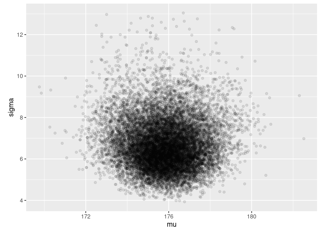
Y ahora extraemos algunas replicaciones de la posterior predictiva:
y_sim_tbl <- ajuste$draws("y_sim") %>% as_draws_df() %>%
  pivot_longer(cols = starts_with("y_sim"), "nombre") %>%
  separate(nombre, c("nombre", "n_obs", "vacio"), "[\\[\\]]") %>%
  select(-nombre, -vacio) %>%
  filter(.chain == 1, .iteration < 12) %>%
  select(.iteration, value) %>%
  bind_rows(tibble(.iteration = 12, value = round(cantantes$estatura_cm, 0)))
## Warning: Dropping 'draws_df' class as required metadata was removed.## Error in `pivot_longer()`:
## ! Arguments in `...` must be used.
## ✖ Problematic argument:
## • ..1 = "nombre"
## ℹ Did you misspell an argument name?ggplot(y_sim_tbl, aes(sample = value)) +
geom_qq() +
facet_wrap(~ .iteration)## Error in eval(expr, envir, enclos): object 'y_sim_tbl' not found13.0.1 Ejemplo: exámenes
sim_formas <- function(p_azar, p_corr){
  tipo <- rbinom(1, 1, 1 - p_azar)
  if(tipo==0){
    # al azar
    x <- rbinom(1, 10, 1/5)
  } else {
    # no al azar
    x <- rbinom(1, 10, p_corr)
  }
  x
}
set.seed(12)
muestra_1 <- map_dbl(1:200, ~ sim_formas(0.35, 0.5))mod_informado## // Ejemplo de estimación del máximo de uniforme
## data {
## int n; // número de observaciones
## array[n] int y; //datos observados
## }
##
##
## parameters {
## real<lower=0, upper=1> theta_azar;
## real<lower=0, upper=1> theta_corr;
## }
##
## model {
## // inicial
## theta_azar ~ beta(1, 5);
## theta_corr ~ beta(7, 3);
## // en este caso, agregamos términos directamente a la log posterior
## for(i in 1:n){
## target+= log_sum_exp(
## log(theta_azar) + binomial_lpmf(y[i] | 10, 0.20),
## log(1 - theta_azar) + binomial_lpmf(y[i] | 10, theta_corr));
## }
## }Pasamos datos y muestreamos
set.seed(3413)
datos_lista <- list(n = length(muestra_1), y = muestra_1)
ajuste <- mod_informado$sample(
  data = datos_lista,
  seed = 1234,
  chains = 4,
  iter_warmup = 4000,
  iter_sampling = 4000,
  refresh = 2000)
## Running MCMC with 4 sequential chains...
##
## Chain 1 Iteration: 1 / 8000 [ 0%] (Warmup)
## Chain 1 Iteration: 2000 / 8000 [ 25%] (Warmup)
## Chain 1 Iteration: 4000 / 8000 [ 50%] (Warmup)
## Chain 1 Iteration: 4001 / 8000 [ 50%] (Sampling)
## Chain 1 Iteration: 6000 / 8000 [ 75%] (Sampling)
## Chain 1 Iteration: 8000 / 8000 [100%] (Sampling)
## Chain 1 finished in 2.1 seconds.
## Chain 2 Iteration: 1 / 8000 [ 0%] (Warmup)
## Chain 2 Iteration: 2000 / 8000 [ 25%] (Warmup)
## Chain 2 Iteration: 4000 / 8000 [ 50%] (Warmup)
## Chain 2 Iteration: 4001 / 8000 [ 50%] (Sampling)
## Chain 2 Iteration: 6000 / 8000 [ 75%] (Sampling)
## Chain 2 Iteration: 8000 / 8000 [100%] (Sampling)
## Chain 2 finished in 2.0 seconds.
## Chain 3 Iteration: 1 / 8000 [ 0%] (Warmup)
## Chain 3 Iteration: 2000 / 8000 [ 25%] (Warmup)
## Chain 3 Iteration: 4000 / 8000 [ 50%] (Warmup)
## Chain 3 Iteration: 4001 / 8000 [ 50%] (Sampling)
## Chain 3 Iteration: 6000 / 8000 [ 75%] (Sampling)
## Chain 3 Iteration: 8000 / 8000 [100%] (Sampling)
## Chain 3 finished in 2.1 seconds.
## Chain 4 Iteration: 1 / 8000 [ 0%] (Warmup)
## Chain 4 Iteration: 2000 / 8000 [ 25%] (Warmup)
## Chain 4 Iteration: 4000 / 8000 [ 50%] (Warmup)
## Chain 4 Iteration: 4001 / 8000 [ 50%] (Sampling)
## Chain 4 Iteration: 6000 / 8000 [ 75%] (Sampling)
## Chain 4 Iteration: 8000 / 8000 [100%] (Sampling)
## Chain 4 finished in 2.2 seconds.
##
## All 4 chains finished successfully.
## Mean chain execution time: 2.1 seconds.
## Total execution time: 8.9 seconds.Checamos diagnósticos:
ajuste$cmdstan_diagnose()## Processing csv files: /tmp/Rtmpv7c8tl/modelo-examenes-202311292013-1-719786.csv, /tmp/Rtmpv7c8tl/modelo-examenes-202311292013-2-719786.csv, /tmp/Rtmpv7c8tl/modelo-examenes-202311292013-3-719786.csv, /tmp/Rtmpv7c8tl/modelo-examenes-202311292013-4-719786.csv
##
## Checking sampler transitions treedepth.
## Treedepth satisfactory for all transitions.
##
## Checking sampler transitions for divergences.
## No divergent transitions found.
##
## Checking E-BFMI - sampler transitions HMC potential energy.
## E-BFMI satisfactory.
##
## Effective sample size satisfactory.
##
## Split R-hat values satisfactory all parameters.
##
## Processing complete, no problems detected.Si no hay problemas, podemos ver el resumen:
resumen <- ajuste$summary()
resumen
## # A tibble: 3 × 10
## variable mean median sd mad q5 q95 rhat ess_bulk
## <chr> <num> <num> <num> <num> <num> <num> <num> <num>
## 1 lp__ -439. -438. 1.00 0.741 -441. -438. 1.00 6789.
## 2 theta_azar 0.375 0.375 0.0468 0.0469 0.298 0.452 1.00 7631.
## 3 theta_corr 0.525 0.525 0.0182 0.0180 0.495 0.555 1.00 8297.
## # ℹ 1 more variable: ess_tail <num>sims_theta_tbl <-
ajuste$draws(c("theta_azar", "theta_corr")) %>%
as_draws_df()
ggplot(sims_theta_tbl, aes(x = theta_azar, y = theta_corr)) +
geom_point(alpha = 0.1)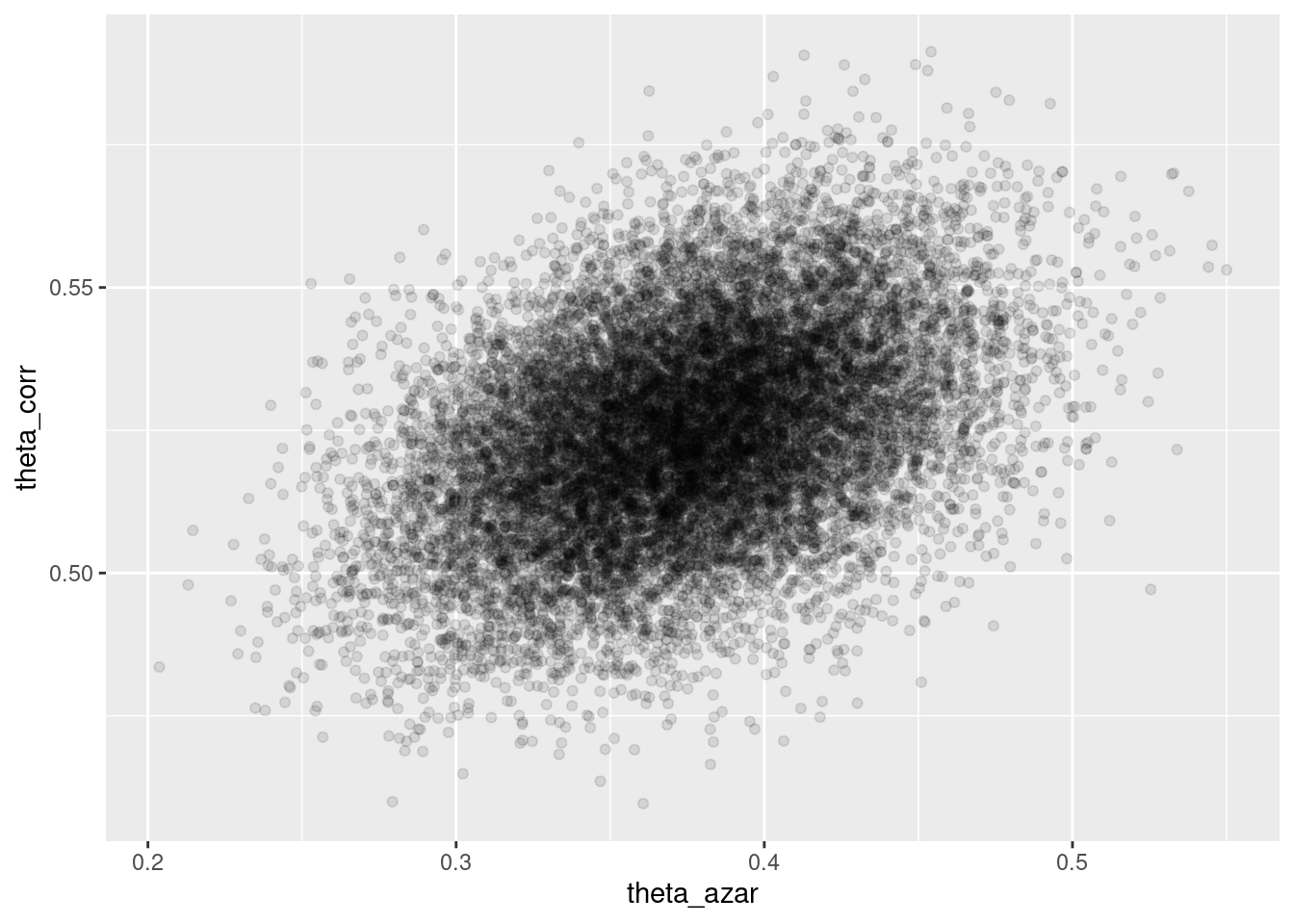
13.1 Ejemplo: exámenes, mal identificado
En este ejemplo cambiamos los parámetros de la simulación y ponemos iniciales poco informativas.
set.seed(12)
muestra_2 <- map_dbl(1:200, ~ sim_formas(0.35, 0.21))mod_no_inf## // Ejemplo de estimación del máximo de uniforme
## data {
## int n; // número de observaciones
## array[n] int y; //datos observados
## }
##
##
## parameters {
## real<lower=0, upper=1> theta_azar;
## real<lower=0, upper=1> theta_corr;
## }
##
## model {
## // inicial
## theta_azar ~ beta(1, 1);
## theta_corr ~ beta(1, 1);
## // en este caso, agregamos términos directamente a la log posterior
## for(i in 1:n){
## target+= log_sum_exp(
## log(theta_azar) + binomial_lpmf(y[i] | 10, 0.20),
## log(1 - theta_azar) + binomial_lpmf(y[i] | 10, theta_corr));
## }
## }Pasamos datos y muestreamos
set.seed(3413)
datos_lista <- list(n = length(muestra_2), y = muestra_2)
ajuste <- mod_no_inf$sample(
data = datos_lista,
seed = 1234,
chains = 4,
iter_warmup = 4000,
iter_sampling = 4000,
refresh = 2000)## Running MCMC with 4 sequential chains...
##
## Chain 1 Iteration: 1 / 8000 [ 0%] (Warmup)
## Chain 1 Iteration: 2000 / 8000 [ 25%] (Warmup)
## Chain 1 Iteration: 4000 / 8000 [ 50%] (Warmup)
## Chain 1 Iteration: 4001 / 8000 [ 50%] (Sampling)
## Chain 1 Iteration: 6000 / 8000 [ 75%] (Sampling)
## Chain 1 Iteration: 8000 / 8000 [100%] (Sampling)
## Chain 1 finished in 2.9 seconds.
## Chain 2 Iteration: 1 / 8000 [ 0%] (Warmup)
## Chain 2 Iteration: 2000 / 8000 [ 25%] (Warmup)
## Chain 2 Iteration: 4000 / 8000 [ 50%] (Warmup)
## Chain 2 Iteration: 4001 / 8000 [ 50%] (Sampling)
## Chain 2 Iteration: 6000 / 8000 [ 75%] (Sampling)
## Chain 2 Iteration: 8000 / 8000 [100%] (Sampling)
## Chain 2 finished in 2.8 seconds.
## Chain 3 Iteration: 1 / 8000 [ 0%] (Warmup)
## Chain 3 Iteration: 2000 / 8000 [ 25%] (Warmup)
## Chain 3 Iteration: 4000 / 8000 [ 50%] (Warmup)
## Chain 3 Iteration: 4001 / 8000 [ 50%] (Sampling)
## Chain 3 Iteration: 6000 / 8000 [ 75%] (Sampling)
## Chain 3 Iteration: 8000 / 8000 [100%] (Sampling)
## Chain 3 finished in 4.9 seconds.
## Chain 4 Iteration: 1 / 8000 [ 0%] (Warmup)
## Chain 4 Iteration: 2000 / 8000 [ 25%] (Warmup)
## Chain 4 Iteration: 4000 / 8000 [ 50%] (Warmup)
## Chain 4 Iteration: 4001 / 8000 [ 50%] (Sampling)
## Chain 4 Iteration: 6000 / 8000 [ 75%] (Sampling)
## Chain 4 Iteration: 8000 / 8000 [100%] (Sampling)
## Chain 4 finished in 2.8 seconds.
##
## All 4 chains finished successfully.
## Mean chain execution time: 3.3 seconds.
## Total execution time: 13.6 seconds.## Warning: 520 of 16000 (3.0%) transitions ended with a divergence.
## See https://mc-stan.org/misc/warnings for details.Y obtenemos mensajes de advertencia (divergencias), lo que implica que los diagnósticos indican que es posible que las cadenas no hayan explorado suficientemente la posterior
ajuste$cmdstan_diagnose()## Processing csv files: /tmp/Rtmpv7c8tl/modelo-examenes-no-inf-202311292013-1-719786.csv, /tmp/Rtmpv7c8tl/modelo-examenes-no-inf-202311292013-2-719786.csv, /tmp/Rtmpv7c8tl/modelo-examenes-no-inf-202311292013-3-719786.csv, /tmp/Rtmpv7c8tl/modelo-examenes-no-inf-202311292013-4-719786.csv
##
## Checking sampler transitions treedepth.
## Treedepth satisfactory for all transitions.
##
## Checking sampler transitions for divergences.
## 520 of 16000 (3.25%) transitions ended with a divergence.
## These divergent transitions indicate that HMC is not fully able to explore the posterior distribution.
## Try increasing adapt delta closer to 1.
## If this doesn't remove all divergences, try to reparameterize the model.
##
## Checking E-BFMI - sampler transitions HMC potential energy.
## E-BFMI satisfactory.
##
## Effective sample size satisfactory.
##
## Split R-hat values satisfactory all parameters.
##
## Processing complete.sims_theta_tbl <-
ajuste$draws(c("theta_azar", "theta_corr")) %>%
as_draws_df()
ggplot(sims_theta_tbl, aes(x = theta_azar, y = theta_corr)) +
geom_point(alpha = 0.1)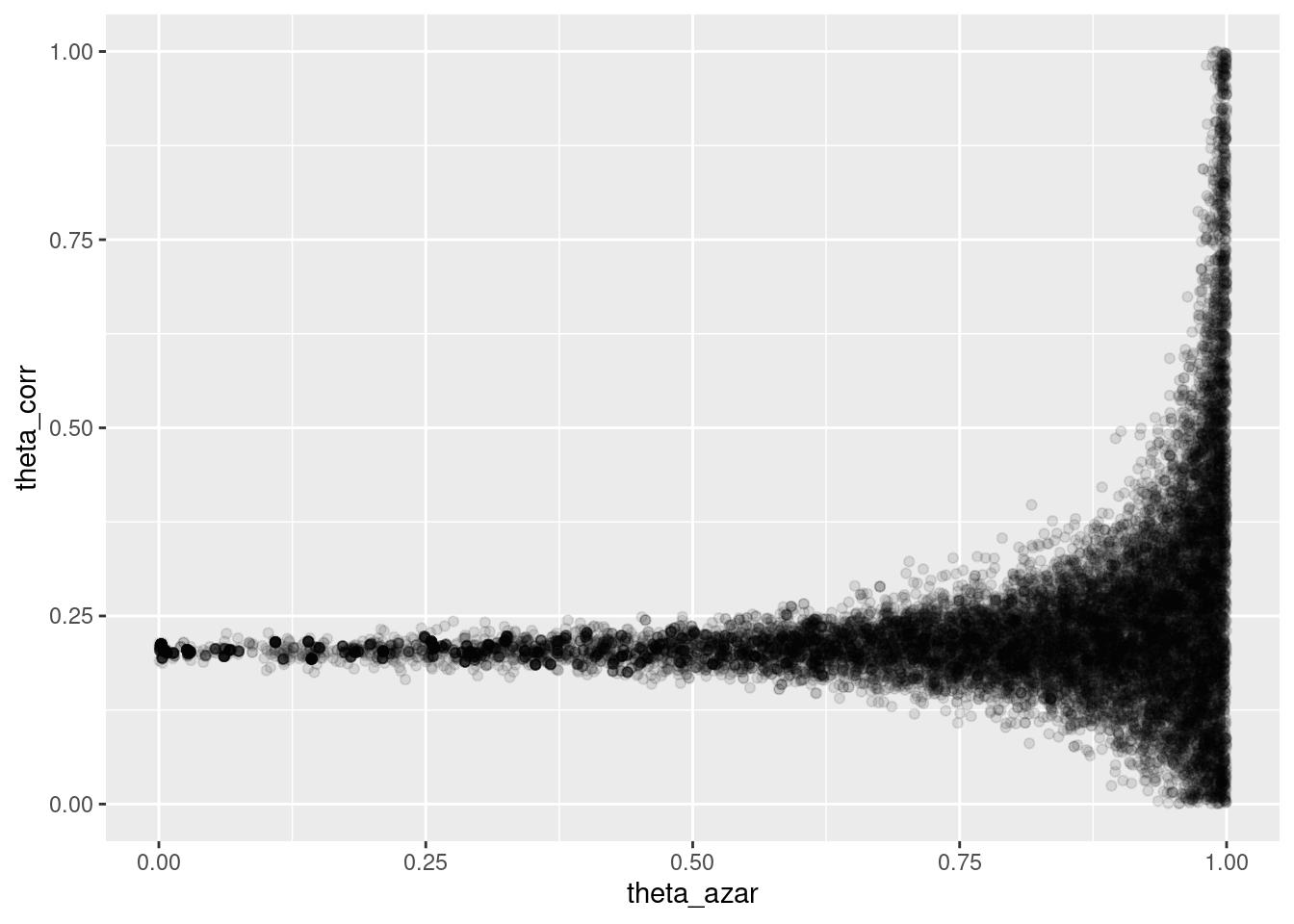
Donde vemos que el problema es serio: cuando \(\theta_{azar}\) es chico, los datos son consistentes con valores de \(\theta_{corr}\) cercanos a 0.2. Pero también es posible que \(\theta_{azar}\) sea grande, y en ese caso tenemos poca información acerca de \(\theta_corr\).
- La geometría de esta posterior hace difícil para el algoritmo establecer el tamaño de paso correcto para explorar adecuadamente esta posterior (con un tamaño de paso chico, explora lentamente, pero si se hace más grande, entonces aparecen problemas numéricos y rechazos en los “embudos” de esta posterior).
- Sin embargo, este resultado generalmente lo rechazaríamos, pues sabemos que una proporción considerable de estudiantes no contesta al azar.
Si corremos el modelo informado con la muestra de esta población, obtenemos:
set.seed(3413)
datos_lista <- list(n = length(muestra_2), y = muestra_2)
ajuste <- mod_informado$sample(
data = datos_lista,
seed = 1234,
chains = 4,
iter_warmup = 4000,
iter_sampling = 4000,
refresh = 2000)## Running MCMC with 4 sequential chains...
##
## Chain 1 Iteration: 1 / 8000 [ 0%] (Warmup)
## Chain 1 Iteration: 2000 / 8000 [ 25%] (Warmup)
## Chain 1 Iteration: 4000 / 8000 [ 50%] (Warmup)
## Chain 1 Iteration: 4001 / 8000 [ 50%] (Sampling)
## Chain 1 Iteration: 6000 / 8000 [ 75%] (Sampling)
## Chain 1 Iteration: 8000 / 8000 [100%] (Sampling)
## Chain 1 finished in 2.3 seconds.
## Chain 2 Iteration: 1 / 8000 [ 0%] (Warmup)
## Chain 2 Iteration: 2000 / 8000 [ 25%] (Warmup)
## Chain 2 Iteration: 4000 / 8000 [ 50%] (Warmup)
## Chain 2 Iteration: 4001 / 8000 [ 50%] (Sampling)
## Chain 2 Iteration: 6000 / 8000 [ 75%] (Sampling)
## Chain 2 Iteration: 8000 / 8000 [100%] (Sampling)
## Chain 2 finished in 2.1 seconds.
## Chain 3 Iteration: 1 / 8000 [ 0%] (Warmup)
## Chain 3 Iteration: 2000 / 8000 [ 25%] (Warmup)
## Chain 3 Iteration: 4000 / 8000 [ 50%] (Warmup)
## Chain 3 Iteration: 4001 / 8000 [ 50%] (Sampling)
## Chain 3 Iteration: 6000 / 8000 [ 75%] (Sampling)
## Chain 3 Iteration: 8000 / 8000 [100%] (Sampling)
## Chain 3 finished in 2.1 seconds.
## Chain 4 Iteration: 1 / 8000 [ 0%] (Warmup)
## Chain 4 Iteration: 2000 / 8000 [ 25%] (Warmup)
## Chain 4 Iteration: 4000 / 8000 [ 50%] (Warmup)
## Chain 4 Iteration: 4001 / 8000 [ 50%] (Sampling)
## Chain 4 Iteration: 6000 / 8000 [ 75%] (Sampling)
## Chain 4 Iteration: 8000 / 8000 [100%] (Sampling)
## Chain 4 finished in 2.0 seconds.
##
## All 4 chains finished successfully.
## Mean chain execution time: 2.1 seconds.
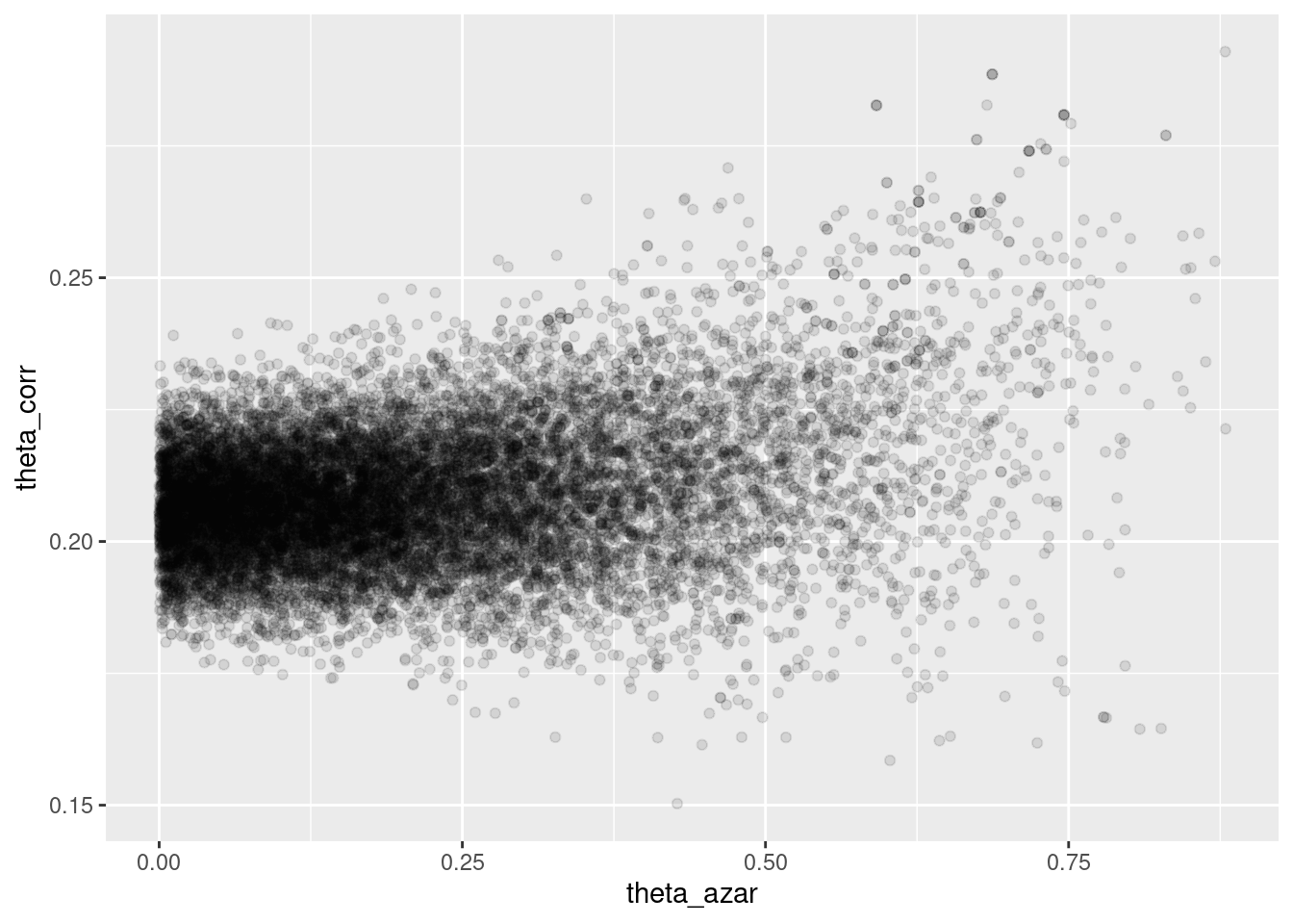
## Total execution time: 8.8 seconds.No tenemos problemas numéricos, y la posterior se ve como sigue:
sims_theta_tbl <-
  ajuste$draws(c("theta_azar", "theta_corr")) %>%
  as_draws_df()
ggplot(sims_theta_tbl, aes(x = theta_azar, y = theta_corr)) +
  geom_point(alpha = 0.1)